🚗Sports Car Price Analysis

🚗Sports Car Price Analysis#

Course Project, UC Irvine, Math 10, F23

✨Introduction#

The project is about analyzing the price of sports cars. I am a big fan of sports cars and I’ve been paying very close attention to the models and prices of different brands of sports cars. Therefore, I think it will be very interesting to analysis this dataset .

I am going analyze the dataset to answer the folllowing questions: 1.Does the configuration of the car have anything to do with the price?( Based on this dataset) 2.Can we use those configurations to predict the price of a car?( Based on this dataset) 3.What price appear the most common in this dataframe?

import pandas as pd
import seaborn as sns
import numpy as np
import altair as alt
import matplotlib.pyplot as plt
from sklearn.tree import plot_tree
from sklearn.linear_model import LinearRegression
from sklearn.linear_model import LogisticRegression
from sklearn.tree import DecisionTreeClassifier
from sklearn.cluster import KMeans
from sklearn.decomposition import PCA
from sklearn.model_selection import train_test_split

🚗Defination and Description#

All the explanations are come from Kaggle websit:https://www.kaggle.com/datasets/rkiattisak/sports-car-prices-dataset

Here are some brief explanations of the columns in this dataset: Car Make—The make of the sports car(The brands of sports cars) Car Model—The model of the sports car Year—The year of production of the sports car Engine Size (L)—The size of the sports car’s engine in liters Horsepower—he horsepower of the sports car Torque (lb-ft)—The torque of the sports car in pound-feet 0-60 MPH Time—The time it takes for the sports car to accelerate from 0 to 60 miles per hour Price (in USD)—The price of the sports car in US dollars

🚗Overview of Dataset#

Load the dataset and name it “df”.

df = pd.read_csv("Sportcarprice.csv") 
df

	Car Make	Car Model	Year	Engine Size (L)	Horsepower	Torque (lb-ft)	0-60 MPH Time (seconds)	Price (in USD)
0	Porsche	911	2022	3	379	331	4	101,200
1	Lamborghini	Huracan	2021	5.2	630	443	2.8	274,390
2	Ferrari	488 GTB	2022	3.9	661	561	3	333,750
3	Audi	R8	2022	5.2	562	406	3.2	142,700
4	McLaren	720S	2021	4	710	568	2.7	298,000
...	...	...	...	...	...	...	...	...
1002	Koenigsegg	Jesko	2022	5	1280	1106	2.5	3,000,000
1003	Lotus	Evija	2021	Electric Motor	1972	1254	2	2,000,000
1004	McLaren	Senna	2021	4	789	590	2.7	1,000,000
1005	Pagani	Huayra	2021	6	764	738	3	2,600,000
1006	Rimac	Nevera	2021	Electric Motor	1888	1696	1.85	2,400,000

1007 rows × 8 columns

🧹Data Cleaning#

Check the shape of the dataframe.

df.shape

(1007, 8)

Now there are 995 rows and 8 columns in the dataset.

Check is there is any missing values in the dataset.

df.isna().any()

Car Make                   False
Car Model                  False
Year                       False
Engine Size (L)             True
Horsepower                 False
Torque (lb-ft)              True
0-60 MPH Time (seconds)    False
Price (in USD)             False
dtype: bool

We can see there are 2 columns contain missing value: Engine Size(L) and Torque.

Now, remove the rows that contain the missing values.

df=df.dropna(axis=0)
df

	Car Make	Car Model	Year	Engine Size (L)	Horsepower	Torque (lb-ft)	0-60 MPH Time (seconds)	Price (in USD)
0	Porsche	911	2022	3	379	331	4	101,200
1	Lamborghini	Huracan	2021	5.2	630	443	2.8	274,390
2	Ferrari	488 GTB	2022	3.9	661	561	3	333,750
3	Audi	R8	2022	5.2	562	406	3.2	142,700
4	McLaren	720S	2021	4	710	568	2.7	298,000
...	...	...	...	...	...	...	...	...
1002	Koenigsegg	Jesko	2022	5	1280	1106	2.5	3,000,000
1003	Lotus	Evija	2021	Electric Motor	1972	1254	2	2,000,000
1004	McLaren	Senna	2021	4	789	590	2.7	1,000,000
1005	Pagani	Huayra	2021	6	764	738	3	2,600,000
1006	Rimac	Nevera	2021	Electric Motor	1888	1696	1.85	2,400,000

995 rows × 8 columns

Check the shape of “df” again.

df.shape

(995, 8)

After removing the missing value, there are 995 rows and 8 columns in this dataset.

👀Observing the Dataset#

Check the data type of each column.

df.dtypes

Car Make                   object
Car Model                  object
Year                        int64
Engine Size (L)            object
Horsepower                 object
Torque (lb-ft)             object
0-60 MPH Time (seconds)    object
Price (in USD)             object
dtype: object

Change the type of Price from “object” to “integer”. For this code, I got help from datacampe: https://www.datacamp.com/tutorial/python-data-type-conversion

df['Price (in USD)'] = df['Price (in USD)'].str.replace(',', '').astype(int)
df

/tmp/ipykernel_207/217902949.py:1: SettingWithCopyWarning: 
A value is trying to be set on a copy of a slice from a DataFrame.
Try using .loc[row_indexer,col_indexer] = value instead

See the caveats in the documentation: https://pandas.pydata.org/pandas-docs/stable/user_guide/indexing.html#returning-a-view-versus-a-copy
  df['Price (in USD)'] = df['Price (in USD)'].str.replace(',', '').astype(int)

	Car Make	Car Model	Year	Engine Size (L)	Horsepower	Torque (lb-ft)	0-60 MPH Time (seconds)	Price (in USD)
0	Porsche	911	2022	3	379	331	4	101200
1	Lamborghini	Huracan	2021	5.2	630	443	2.8	274390
2	Ferrari	488 GTB	2022	3.9	661	561	3	333750
3	Audi	R8	2022	5.2	562	406	3.2	142700
4	McLaren	720S	2021	4	710	568	2.7	298000
...	...	...	...	...	...	...	...	...
1002	Koenigsegg	Jesko	2022	5	1280	1106	2.5	3000000
1003	Lotus	Evija	2021	Electric Motor	1972	1254	2	2000000
1004	McLaren	Senna	2021	4	789	590	2.7	1000000
1005	Pagani	Huayra	2021	6	764	738	3	2600000
1006	Rimac	Nevera	2021	Electric Motor	1888	1696	1.85	2400000

995 rows × 8 columns

Check how many sports car brands are here in this dataset.

df["Car Make"].unique ()

array(['Porsche', 'Lamborghini', 'Ferrari', 'Audi', 'McLaren', 'BMW',
       'Mercedes-Benz', 'Chevrolet', 'Ford', 'Nissan', 'Aston Martin',
       'Bugatti', 'Dodge', 'Jaguar', 'Koenigsegg', 'Lexus', 'Lotus',
       'Maserati', 'Alfa Romeo', 'Ariel', 'Bentley', 'Mercedes-AMG',
       'Pagani', 'Polestar', 'Rimac', 'Acura', 'Mazda', 'Rolls-Royce',
       'Tesla', 'Toyota', 'W Motors', 'Shelby', 'TVR', 'Subaru',
       'Pininfarina', 'Kia', 'Alpine', 'Ultima'], dtype=object)

len(df["Car Make"].unique ())

df["Car Make"].value_counts()

Porsche          86
McLaren          75
Audi             71
Lamborghini      66
BMW              63
Chevrolet        60
Ferrari          55
Mercedes-Benz    54
Aston Martin     50
Ford             48
Dodge            41
Nissan           37
Lotus            34
Jaguar           30
Lexus            26
Bentley          25
Maserati         24
Bugatti          23
Alfa Romeo       16
Acura            16
Koenigsegg       15
Tesla            14
Pagani           12
Rimac            11
Mercedes-AMG     11
Rolls-Royce      10
Toyota            5
Subaru            3
W Motors          3
TVR               2
Pininfarina       2
Polestar          1
Shelby            1
Ariel             1
Alpine            1
Mazda             1
Ultima            1
Kia               1
Name: Car Make, dtype: int64

I just want the top 10 brands to be appeared in the dataframe.Make a new dataframe contain only the top 10 sports car brand and name it df2.

top_brands = df["Car Make"].value_counts().index[:10]
top_brands

Index(['Porsche', 'McLaren', 'Audi', 'Lamborghini', 'BMW', 'Chevrolet',
       'Ferrari', 'Mercedes-Benz', 'Aston Martin', 'Ford'],
      dtype='object')

df2=df[df["Car Make"].isin(top_brands)]
df2

	Car Make	Car Model	Year	Engine Size (L)	Horsepower	Torque (lb-ft)	0-60 MPH Time (seconds)	Price (in USD)
0	Porsche	911	2022	3	379	331	4	101200
1	Lamborghini	Huracan	2021	5.2	630	443	2.8	274390
2	Ferrari	488 GTB	2022	3.9	661	561	3	333750
3	Audi	R8	2022	5.2	562	406	3.2	142700
4	McLaren	720S	2021	4	710	568	2.7	298000
...	...	...	...	...	...	...	...	...
996	Mercedes-Benz	SLS AMG	2021	6.3	622	468	3.6	254500
997	Chevrolet	Camaro	2021	6.2	455	455	4	25000
998	Ford	Mustang	2021	2.3	310	350	5.3	27205
1000	Aston Martin	Vantage	2021	4	503	505	3.6	146000
1004	McLaren	Senna	2021	4	789	590	2.7	1000000

628 rows × 8 columns

Ckeck the shape of df2.

df2.shape

(628, 8)

🤔Explore different configurations of cars with the car price#

Generally speaking, the horsepower of a sport car and its price are directly proportional in our perception. The better the horsepower of the car, the more expensive it might be. Therefore, I wanna to explore if the horsepower is also increase as the price increase. I will use single variabel linear regression here first.

I Linear Regression Model#

First, I wanna to generate an Altair plot to show the relationsihp between hoursepower and price, with the color defined by differnt sport car brands.

c1=alt.Chart(df2).mark_circle().encode(
    x="Horsepower",
    y="Price (in USD)",
    color="Car Make"
)
c1

We can see that the price is increasing with horsepower in general but not really obvious. How about to use linear regression to find a line to find the relationship between Price and Horsepower?

reg = LinearRegression()
X = df2[["Horsepower"]]
y = df2["Price (in USD)"]
X_train, X_test, y_train, y_test = train_test_split(X, y, test_size=0.3, random_state=42)
reg.fit(X_train,y_train)

LinearRegression()

In a Jupyter environment, please rerun this cell to show the HTML representation or trust the notebook.
On GitHub, the HTML representation is unable to render, please try loading this page with nbviewer.org.

reg.coef_

array([1021.84613349])

reg.intercept_

-375922.44599840173

reg.score(X_test,y_test)

0.294063539733909

c2=alt.Chart(df2).mark_line().encode(
    x = "Horsepower",
    y = "Price (in USD)"
)
c1+c2

✍️Linear Regression Conclusion:(Horsepower and Price)#

Since the coefficient of this linear regresssion is positive(1021.84613349),this means that the horsepower is proportional to the price of the car. However,the score of this linear model is low (about 0.29),which means that the linear regression model is not capturing the relationship between the horsepower and the price very well.

II Logistics Regression Model#

Then, I want to use Horsepower and Torque to predict the price level of a sport car.

Frist, I divided the price into 3 level: low ,median and high,based on the interquartile range( upper quartile and lower quartile). This code is learned by me from Codecademy: https://www.codecademy.com/learn/learn-statistics-with-python/modules/quartiles-quantiles-and-interquartile-range/cheatsheet

#Extra
q1 = df2['Price (in USD)'].quantile(0.25)
q1

71800.0

#Extra
q3 = df2['Price (in USD)'].quantile(0.75)
q3

256500.0

Then, I add the “pricelevel” column to the df2. For this code, I have get the help from AI tool.

#Extra
df2["pricelevel"] = np.where(df2["Price (in USD)"] <= q1, "low", np.where(df2["Price (in USD)"] >=q3, "high", "mid"))
df2

/tmp/ipykernel_207/314215083.py:2: SettingWithCopyWarning: 
A value is trying to be set on a copy of a slice from a DataFrame.
Try using .loc[row_indexer,col_indexer] = value instead

See the caveats in the documentation: https://pandas.pydata.org/pandas-docs/stable/user_guide/indexing.html#returning-a-view-versus-a-copy
  df2["pricelevel"] = np.where(df2["Price (in USD)"] <= q1, "low", np.where(df2["Price (in USD)"] >=q3, "high", "mid"))

	Car Make	Car Model	Year	Engine Size (L)	Horsepower	Torque (lb-ft)	0-60 MPH Time (seconds)	Price (in USD)	pricelevel
0	Porsche	911	2022	3	379	331	4	101200	mid
1	Lamborghini	Huracan	2021	5.2	630	443	2.8	274390	high
2	Ferrari	488 GTB	2022	3.9	661	561	3	333750	high
3	Audi	R8	2022	5.2	562	406	3.2	142700	mid
4	McLaren	720S	2021	4	710	568	2.7	298000	high
...	...	...	...	...	...	...	...	...	...
996	Mercedes-Benz	SLS AMG	2021	6.3	622	468	3.6	254500	mid
997	Chevrolet	Camaro	2021	6.2	455	455	4	25000	low
998	Ford	Mustang	2021	2.3	310	350	5.3	27205	low
1000	Aston Martin	Vantage	2021	4	503	505	3.6	146000	mid
1004	McLaren	Senna	2021	4	789	590	2.7	1000000	high

628 rows × 9 columns

alt.Chart(df2).mark_circle().encode(
    x=alt.X("Horsepower", scale=alt.Scale(zero=False)),
    y=alt.Y("Torque (lb-ft)", scale=alt.Scale(zero=False)),
    color="pricelevel:N"
).properties(
    width=400, 
    height=300 
).properties(
    title = 'Price Level '
)

Now, I am going to fit the logistics regression model on this data.

cols = ["Horsepower", "Torque (lb-ft)"]
clf = LogisticRegression()
from sklearn.model_selection import train_test_split
X_train, X_test, y_train, y_test = train_test_split(df2[cols], df2["pricelevel"], test_size=0.2, random_state=41)
clf.fit(X_train, y_train)

LogisticRegression()

In a Jupyter environment, please rerun this cell to show the HTML representation or trust the notebook.
On GitHub, the HTML representation is unable to render, please try loading this page with nbviewer.org.

clf.score(X_test, y_test)

0.7222222222222222

The score of this prediciton is pretty good that the model correctly predicted the price for about 72% of the data.

clf.classes_

array(['high', 'low', 'mid'], dtype=object)

clf.coef_

array([[ 0.04434716, -0.01891043],
       [-0.0358422 ,  0.01738233],
       [-0.00850496,  0.0015281 ]])

Add the “pred” column to the dataframe to store the prediction results.

df2['pred'] = clf.predict(df2[cols])
df2

/tmp/ipykernel_207/1051173615.py:2: SettingWithCopyWarning: 
A value is trying to be set on a copy of a slice from a DataFrame.
Try using .loc[row_indexer,col_indexer] = value instead

See the caveats in the documentation: https://pandas.pydata.org/pandas-docs/stable/user_guide/indexing.html#returning-a-view-versus-a-copy
  df2['pred'] = clf.predict(df2[cols])

	Car Make	Car Model	Year	Engine Size (L)	Horsepower	Torque (lb-ft)	0-60 MPH Time (seconds)	Price (in USD)	pricelevel	pred
0	Porsche	911	2022	3	379	331	4	101200	mid	low
1	Lamborghini	Huracan	2021	5.2	630	443	2.8	274390	high	high
2	Ferrari	488 GTB	2022	3.9	661	561	3	333750	high	mid
3	Audi	R8	2022	5.2	562	406	3.2	142700	mid	mid
4	McLaren	720S	2021	4	710	568	2.7	298000	high	high
...	...	...	...	...	...	...	...	...	...	...
996	Mercedes-Benz	SLS AMG	2021	6.3	622	468	3.6	254500	mid	mid
997	Chevrolet	Camaro	2021	6.2	455	455	4	25000	low	low
998	Ford	Mustang	2021	2.3	310	350	5.3	27205	low	low
1000	Aston Martin	Vantage	2021	4	503	505	3.6	146000	mid	mid
1004	McLaren	Senna	2021	4	789	590	2.7	1000000	high	high

628 rows × 10 columns

alt.Chart(df2).mark_circle().encode(
    x=alt.X("Horsepower", scale=alt.Scale(zero=False)),
    y=alt.Y("Torque (lb-ft)", scale=alt.Scale(zero=False)),
    color="pred"
).properties(
    width=400, 
    height=300 
).properties(
    title = 'Price Level Prediction'
)

✍️Logistic Regression Conclusion#

The predictions of the price by using Horsepower and Torque (lb-ft) in this ✍️Logistic Regression model is reliable with a score about 72% of accuracy.

III Decision Tree Classifier#

Here, I want to see if I can use the three configurations (“Engine Size (L)”,”Horsepower”, “Torque (lb-ft)”) to decide which brand the car is. So I am going to use Decision Tree Model here to do this.

First, I find out that some of the data in the Engine Size column are not flote numbers. So I will first delete all the rows where the column “‘Engine Size (L)’” is not a flote number. For this code, I get help from educative: https://www.educative.io/answers/what-is-the-tonumeric-function-in-pandas

#Extra
df2['Engine Size (L)'] = pd.to_numeric(df2['Engine Size (L)'], errors='coerce')
df2 = df2.dropna(subset=['Engine Size (L)'])
df2

/tmp/ipykernel_207/3673321606.py:2: SettingWithCopyWarning: 
A value is trying to be set on a copy of a slice from a DataFrame.
Try using .loc[row_indexer,col_indexer] = value instead

See the caveats in the documentation: https://pandas.pydata.org/pandas-docs/stable/user_guide/indexing.html#returning-a-view-versus-a-copy
  df2['Engine Size (L)'] = pd.to_numeric(df2['Engine Size (L)'], errors='coerce')

	Car Make	Car Model	Year	Engine Size (L)	Horsepower	Torque (lb-ft)	0-60 MPH Time (seconds)	Price (in USD)	pricelevel	pred
0	Porsche	911	2022	3.0	379	331	4	101200	mid	low
1	Lamborghini	Huracan	2021	5.2	630	443	2.8	274390	high	high
2	Ferrari	488 GTB	2022	3.9	661	561	3	333750	high	mid
3	Audi	R8	2022	5.2	562	406	3.2	142700	mid	mid
4	McLaren	720S	2021	4.0	710	568	2.7	298000	high	high
...	...	...	...	...	...	...	...	...	...	...
996	Mercedes-Benz	SLS AMG	2021	6.3	622	468	3.6	254500	mid	mid
997	Chevrolet	Camaro	2021	6.2	455	455	4	25000	low	low
998	Ford	Mustang	2021	2.3	310	350	5.3	27205	low	low
1000	Aston Martin	Vantage	2021	4.0	503	505	3.6	146000	mid	mid
1004	McLaren	Senna	2021	4.0	789	590	2.7	1000000	high	high

612 rows × 10 columns

Now, I am going to use the Decision Tree classifier to divide the data.

cols2 = ["Engine Size (L)","Horsepower", "Torque (lb-ft)"]
clf2 = DecisionTreeClassifier(max_leaf_nodes=8, random_state=40)
X_train, X_test, y_train, y_test = train_test_split(df2[cols2], df2["Car Make"], test_size=0.2, random_state=39)

clf2.fit(X_train, y_train)

DecisionTreeClassifier(max_leaf_nodes=8, random_state=40)

In a Jupyter environment, please rerun this cell to show the HTML representation or trust the notebook.
On GitHub, the HTML representation is unable to render, please try loading this page with nbviewer.org.

clf2.score(X_test, y_test)

0.5365853658536586

The score of the Decision Tree Model is about 0.53 which means it accurately predict 53% of the brands of cars here. Now I am going to plot the graph of the decision treee.

plt.figure(figsize=(12, 8))
plot_tree(clf2, 
                feature_names=clf2.feature_names_in_,
                class_names=clf2.classes_,
                filled=True)

[Text(0.4444444444444444, 0.9285714285714286, 'Torque (lb-ft) <= 343.0\ngini = 0.898\nsamples = 489\nvalue = [45, 50, 50, 53, 47, 39, 51, 57, 36, 61]\nclass = Porsche'),
 Text(0.3333333333333333, 0.7857142857142857, 'gini = 0.111\nsamples = 51\nvalue = [0, 0, 3, 0, 0, 0, 0, 0, 0, 48]\nclass = Porsche'),
 Text(0.5555555555555556, 0.7857142857142857, 'Engine Size (L) <= 5.35\ngini = 0.893\nsamples = 438\nvalue = [45, 50, 47, 53, 47, 39, 51, 57, 36, 13]\nclass = McLaren'),
 Text(0.3333333333333333, 0.6428571428571429, 'Torque (lb-ft) <= 409.5\ngini = 0.872\nsamples = 337\nvalue = [45, 50, 47, 0, 45, 39, 17, 57, 24, 13]\nclass = McLaren'),
 Text(0.2222222222222222, 0.5, 'gini = 0.541\nsamples = 56\nvalue = [0, 20, 32, 0, 0, 0, 0, 0, 4, 0]\nclass = BMW'),
 Text(0.4444444444444444, 0.5, 'Torque (lb-ft) <= 556.5\ngini = 0.863\nsamples = 281\nvalue = [45, 30, 15, 0, 45, 39, 17, 57, 20, 13]\nclass = McLaren'),
 Text(0.3333333333333333, 0.35714285714285715, 'Torque (lb-ft) <= 540.5\ngini = 0.79\nsamples = 159\nvalue = [29, 8, 15, 0, 2, 38, 1, 50, 15, 1]\nclass = McLaren'),
 Text(0.2222222222222222, 0.21428571428571427, 'Horsepower <= 542.5\ngini = 0.74\nsamples = 120\nvalue = [29, 8, 5, 0, 2, 9, 1, 50, 15, 1]\nclass = McLaren'),
 Text(0.1111111111111111, 0.07142857142857142, 'gini = 0.744\nsamples = 59\nvalue = [24, 8, 5, 0, 0, 9, 0, 0, 12, 1]\nclass = Aston Martin'),
 Text(0.3333333333333333, 0.07142857142857142, 'gini = 0.318\nsamples = 61\nvalue = [5, 0, 0, 0, 2, 0, 1, 50, 3, 0]\nclass = McLaren'),
 Text(0.4444444444444444, 0.21428571428571427, 'gini = 0.381\nsamples = 39\nvalue = [0, 0, 10, 0, 0, 29, 0, 0, 0, 0]\nclass = Ford'),
 Text(0.5555555555555556, 0.35714285714285715, 'gini = 0.794\nsamples = 122\nvalue = [16, 22, 0, 0, 43, 1, 16, 7, 5, 12]\nclass = Ferrari'),
 Text(0.7777777777777778, 0.6428571428571429, 'Horsepower <= 689.5\ngini = 0.597\nsamples = 101\nvalue = [0, 0, 0, 53, 2, 0, 34, 0, 12, 0]\nclass = Chevrolet'),
 Text(0.6666666666666666, 0.5, 'gini = 0.301\nsamples = 65\nvalue = [0, 0, 0, 53, 0, 0, 0, 0, 12, 0]\nclass = Chevrolet'),
 Text(0.8888888888888888, 0.5, 'gini = 0.105\nsamples = 36\nvalue = [0, 0, 0, 0, 2, 0, 34, 0, 0, 0]\nclass = Lamborghini')]

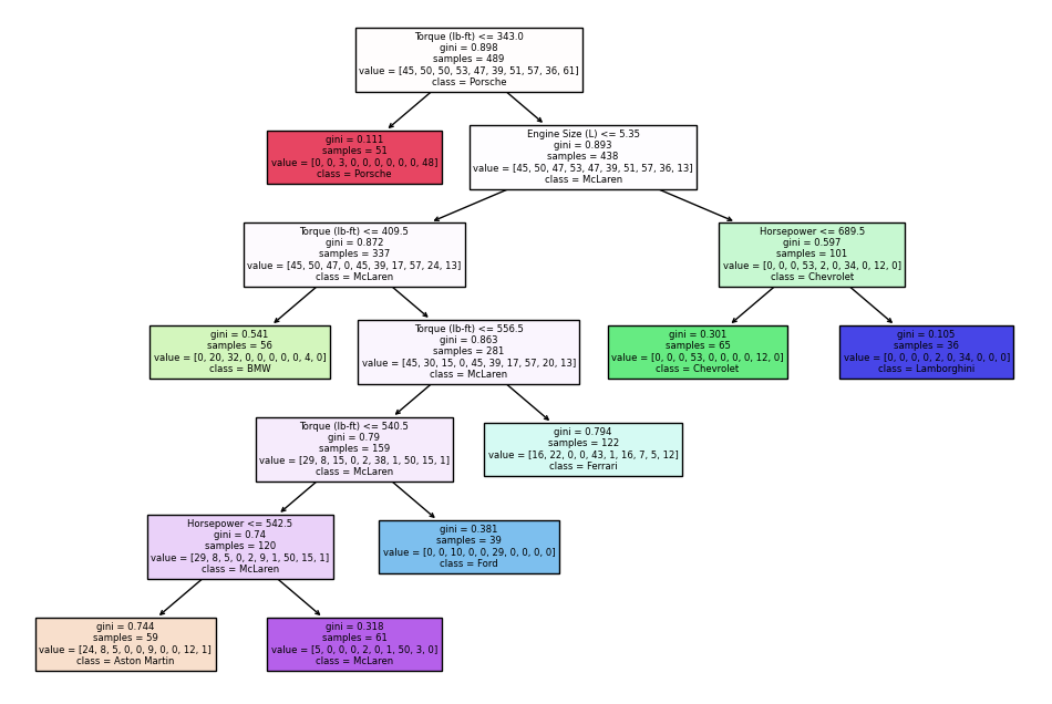
../../_images/a8e071fbba9fac04c64953e28fff087f71880d0f1f70ad3c8f67789fc6fb4345.png

✍️Decision Tree Classifier Conclusion#

The decision tree is about to classify the brands of cars accoring to the car’s Engine Size (L),Horsepower and Torque (lb-ft). However, we can see that the gini score of them are not really good. If we wan to find a more accurate Classifier, I suggest to increase the number of nudes and the depth of the decision tree. Also, don’t forget to be aware of overfitting.

Kmeans#

Here, I want to use Engine Size (L),Horsepower and Torque (lb-ft) to see if I can classify the brands of cars. I will use the Kmeans, and also use PCA to decompose the dimensions of the data.

kmeans = KMeans(n_clusters=3, random_state=0)
y_km = kmeans.fit_predict(df2[cols2])

y_km

array([0, 1, 1, 0, 1, 1, 0, 0, 1, 1, 0, 1, 0, 1, 2, 1, 1, 0, 1, 1, 1, 1,
       1, 0, 1, 1, 0, 1, 2, 0, 0, 0, 0, 0, 0, 0, 0, 1, 1, 0, 1, 1, 0, 0,
       0, 0, 1, 1, 1, 0, 0, 0, 0, 0, 1, 0, 1, 0, 0, 1, 1, 0, 0, 1, 2, 0,
       1, 0, 1, 1, 1, 1, 0, 1, 1, 1, 1, 0, 0, 1, 1, 1, 1, 0, 0, 1, 1, 1,
       1, 0, 0, 0, 0, 1, 1, 0, 0, 0, 1, 0, 0, 0, 1, 1, 0, 1, 0, 0, 1, 0,
       0, 0, 0, 1, 2, 1, 1, 0, 1, 0, 1, 1, 1, 0, 0, 1, 0, 1, 0, 1, 1, 1,
       1, 0, 1, 1, 0, 1, 1, 1, 0, 0, 1, 1, 2, 1, 1, 0, 1, 1, 1, 1, 1, 0,
       1, 0, 1, 0, 1, 0, 0, 0, 1, 1, 0, 1, 0, 1, 1, 0, 0, 0, 0, 1, 1, 2,
       0, 1, 1, 0, 0, 0, 1, 1, 1, 2, 1, 0, 0, 1, 1, 1, 1, 1, 1, 1, 1, 0,
       1, 1, 1, 0, 1, 1, 1, 1, 1, 0, 1, 0, 0, 1, 1, 0, 0, 0, 0, 0, 1, 0,
       1, 1, 1, 1, 1, 1, 0, 0, 0, 0, 0, 0, 1, 1, 0, 1, 1, 1, 0, 0, 1, 1,
       1, 1, 0, 1, 1, 0, 1, 0, 0, 0, 0, 0, 2, 1, 0, 1, 0, 0, 1, 0, 0, 0,
       0, 0, 0, 1, 1, 0, 0, 0, 0, 1, 2, 0, 1, 0, 1, 1, 1, 1, 1, 1, 0, 0,
       0, 0, 1, 1, 0, 0, 1, 1, 0, 0, 1, 1, 0, 1, 1, 1, 1, 1, 1, 1, 1, 1,
       1, 1, 0, 0, 1, 0, 1, 1, 2, 1, 0, 1, 0, 1, 1, 0, 0, 1, 1, 1, 1, 1,
       0, 1, 1, 1, 1, 1, 0, 1, 0, 0, 1, 1, 0, 0, 0, 0, 0, 1, 1, 0, 1, 2,
       1, 1, 1, 2, 1, 0, 0, 1, 0, 1, 1, 1, 0, 1, 1, 1, 1, 1, 0, 0, 0, 1,
       2, 1, 1, 0, 1, 1, 1, 1, 0, 1, 0, 0, 0, 1, 1, 1, 0, 0, 1, 0, 1, 0,
       1, 2, 1, 1, 0, 1, 1, 1, 1, 2, 2, 1, 1, 1, 1, 0, 0, 0, 1, 1, 0, 1,
       0, 0, 0, 0, 1, 2, 1, 1, 1, 1, 1, 1, 1, 1, 1, 0, 0, 0, 1, 1, 0, 1,
       0, 1, 0, 1, 1, 1, 1, 1, 1, 0, 1, 1, 2, 1, 1, 0, 1, 1, 1, 1, 1, 1,
       0, 1, 0, 1, 0, 0, 1, 2, 0, 1, 0, 1, 0, 1, 0, 1, 1, 1, 2, 1, 1, 1,
       1, 0, 0, 0, 1, 0, 0, 1, 2, 0, 0, 0, 0, 0, 0, 0, 0, 1, 0, 1, 0, 0,
       1, 1, 1, 1, 1, 0, 0, 0, 0, 1, 1, 1, 1, 0, 0, 0, 0, 0, 1, 1, 0, 0,
       0, 1, 0, 1, 1, 1, 1, 1, 0, 1, 1, 0, 1, 0, 0, 1, 1, 1, 1, 0, 0, 0,
       0, 1, 1, 1, 0, 0, 0, 1, 2, 0, 0, 0, 0, 0, 1, 1, 0, 0, 1, 0, 0, 0,
       0, 0, 0, 0, 1, 1, 1, 1, 1, 0, 1, 1, 1, 0, 1, 2, 1, 1, 0, 0, 1, 1,
       0, 1, 1, 0, 0, 1, 0, 0, 1, 2, 0, 1, 0, 1, 0, 0, 0, 1], dtype=int32)

df2['kmeans_cluster'] = y_km
pca = PCA(n_components=2)
X_pca = pca.fit_transform(df2[cols])
df2[['PC1','PC2']] = X_pca

/tmp/ipykernel_207/727528674.py:1: SettingWithCopyWarning: 
A value is trying to be set on a copy of a slice from a DataFrame.
Try using .loc[row_indexer,col_indexer] = value instead

See the caveats in the documentation: https://pandas.pydata.org/pandas-docs/stable/user_guide/indexing.html#returning-a-view-versus-a-copy
  df2['kmeans_cluster'] = y_km
/tmp/ipykernel_207/727528674.py:4: SettingWithCopyWarning: 
A value is trying to be set on a copy of a slice from a DataFrame.
Try using .loc[row_indexer,col_indexer] = value instead

See the caveats in the documentation: https://pandas.pydata.org/pandas-docs/stable/user_guide/indexing.html#returning-a-view-versus-a-copy
  df2[['PC1','PC2']] = X_pca
/shared-libs/python3.9/py/lib/python3.9/site-packages/pandas/core/indexing.py:1738: SettingWithCopyWarning: 
A value is trying to be set on a copy of a slice from a DataFrame.
Try using .loc[row_indexer,col_indexer] = value instead

See the caveats in the documentation: https://pandas.pydata.org/pandas-docs/stable/user_guide/indexing.html#returning-a-view-versus-a-copy
  self._setitem_single_column(loc, value[:, i].tolist(), pi)

I will plot the graph of about the car brand after decomposition to 2 dimensions :” PC1” and “PC2”

c3= alt.Chart(df2).mark_circle(size = 60).encode(
    x = 'PC1',
    y = 'PC2',
    color = alt.Color('Car Make:N', scale = alt.Scale(scheme='set1')),
    tooltip = ['Price (in USD):N',"Car Make"]
).properties(
    title = 'Car Brands'
)
c3

✍️Kmeans Conclusion#

So we can see there is no obvious pattern by using Kmeans to group those data. Therefore, we can not decide the brand of the car just by using the Engine Size, Horsepower and the Torque.

✨(Extra)Price Count Plot#

For this code reference :https://matplotlib.org/stable/api/_as_gen/matplotlib.pyplot.figure.html

plt.figure(figsize=(30,10))
sns.countplot(x="Price (in USD)", data=df2)
plt.show()

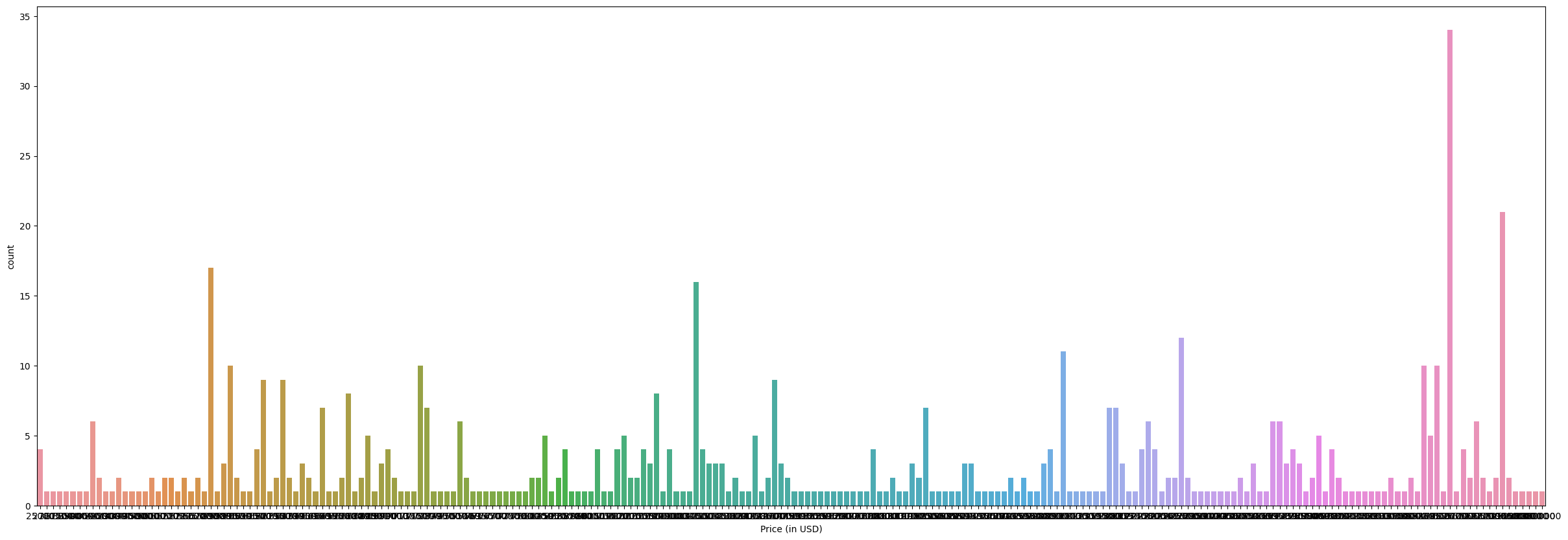
../../_images/e99d3b52b00542ea84b50b72b15eb2c24063aee93632e859d6fbaf093876dd19.png

This plot above shows the Price (in USD) vs the count. We can see that the price that appear the most is highest pink bar. Let’s figuer out which price it is and how many time this price has appeared in this dataframe.

mode_price = df2['Price (in USD)'].value_counts().idxmax()
mode_price

max_count = df2['Price (in USD)'].value_counts().max()
max_count

So, the price that appears the most is $500000. It has appeared 34 times.

📝Summary#

Back to the question at the very top:#

1.Does the configuration of the car have anything to do with the price?( Based on this dataset)#

In my analysis process, I use ‘ Horsepower’ as the configuration and price as the target. And the I find out that there is no obvious relationship between the Horsepower and price of a sport car.

2.Can we use those configurations to predict the price of a car?( Based on this dataset)#

Yes. In my analysis process, I divided the price in to 3 levels: high, mid and low. Then, I use “Horsepower”, “Torque (lb-ft)”as input features and the price level as output, the logistics regression model performed well to predict the price level of the car.

3.What price appear the most in this dataframe?#

$500000 is the most common price of sports car in this dataset. And it has appeared 34 times.

References#

Your code above should include references. Here is some additional space for references.

What is the source of your dataset(s)?

My dataset comes from Kaggle: Sports Car Price Dataset: https://www.kaggle.com/datasets/rkiattisak/sports-car-prices-dataset

List any other references that you found helpful.

The reference of the code about finding the upper quartile and lower quartile: https://www.codecademy.com/learn/learn-statistics-with-python/modules/quartiles-quantiles-and-interquartile-range/cheatsheet
The reference of the code about adding the “priceleve” column is generated by AI tool.
The reference of “to_numeric” function to convert given argument to a numeric type :https://www.educative.io/answers/what-is-the-tonumeric-function-in-pandas
The reference of the “Price Count Plot” part : https://matplotlib.org/stable/api/_as_gen/matplotlib.pyplot.figure.html4.
The reference of the “Change the type of Price from ‘object’ to ‘integer’” part : https://www.datacamp.com/tutorial/python-data-type-conversion
This is the project of a previous student that I have imitated the layout of her/his work. https://christopherdavisuci.github.io/UCI-Math-10-S23/Proj/StudentProjects/LoulouVivianMahfouz.html

🚗Sports Car Price Analysis

Contents

🚗Sports Car Price Analysis#

✨Introduction#

🚗Defination and Description#

🚗Overview of Dataset#

🧹Data Cleaning#

👀Observing the Dataset#

🤔Explore different configurations of cars with the car price#

I Linear Regression Model#

✍️Linear Regression Conclusion:(Horsepower and Price)#

II Logistics Regression Model#

✍️Logistic Regression Conclusion#

III Decision Tree Classifier#

✍️Decision Tree Classifier Conclusion#

Kmeans#

✍️Kmeans Conclusion#

✨(Extra)Price Count Plot#

📝Summary#

Back to the question at the very top:#

1.Does the configuration of the car have anything to do with the price?( Based on this dataset)#

2.Can we use those configurations to predict the price of a car?( Based on this dataset)#

3.What price appear the most in this dataframe?#

References#