Predicting Success of MLB Teams

Predicting Success of MLB Teams#

Author: Eric Cao

Course Project, UC Irvine, Math 10, F23

Introduction#

Among baseball executives and fans, there is much debate about the way a MLB team’s roster should be constructed. Some abide by the slogan “Defense wins championships”, while others place more emphasis on offense. The goal of this project is to apply machine learning methods to a dataset containing teams’ stats to determine which stats, if any, have the largest effect on a team’s success.

Cleaning the Data#

First import all the necessary modules and functions.

import pandas as pd
import numpy as np
import altair as alt
import matplotlib.pyplot as plt
import seaborn as sns
from sklearn.preprocessing import MinMaxScaler
from sklearn.model_selection import train_test_split
from sklearn.linear_model import LinearRegression
from sklearn.ensemble import RandomForestClassifier
import tensorflow as tf
from sklearn.metrics import mean_squared_error, mean_absolute_error, accuracy_score, confusion_matrix, classification_report

2023-12-14 08:52:56.790851: I tensorflow/core/platform/cpu_feature_guard.cc:193] This TensorFlow binary is optimized with oneAPI Deep Neural Network Library (oneDNN) to use the following CPU instructions in performance-critical operations:  AVX2 AVX512F FMA
To enable them in other operations, rebuild TensorFlow with the appropriate compiler flags.
2023-12-14 08:52:57.097621: W tensorflow/stream_executor/platform/default/dso_loader.cc:64] Could not load dynamic library 'libcudart.so.11.0'; dlerror: libcudart.so.11.0: cannot open shared object file: No such file or directory
2023-12-14 08:52:57.097645: I tensorflow/stream_executor/cuda/cudart_stub.cc:29] Ignore above cudart dlerror if you do not have a GPU set up on your machine.
2023-12-14 08:52:57.187274: E tensorflow/stream_executor/cuda/cuda_blas.cc:2981] Unable to register cuBLAS factory: Attempting to register factory for plugin cuBLAS when one has already been registered
2023-12-14 08:52:58.839821: W tensorflow/stream_executor/platform/default/dso_loader.cc:64] Could not load dynamic library 'libnvinfer.so.7'; dlerror: libnvinfer.so.7: cannot open shared object file: No such file or directory
2023-12-14 08:52:58.839909: W tensorflow/stream_executor/platform/default/dso_loader.cc:64] Could not load dynamic library 'libnvinfer_plugin.so.7'; dlerror: libnvinfer_plugin.so.7: cannot open shared object file: No such file or directory
2023-12-14 08:52:58.839919: W tensorflow/compiler/tf2tensorrt/utils/py_utils.cc:38] TF-TRT Warning: Cannot dlopen some TensorRT libraries. If you would like to use Nvidia GPU with TensorRT, please make sure the missing libraries mentioned above are installed properly.

df_raw = pd.read_csv('mlb_teams.csv')
df_raw

	year	league_id	division_id	rank	games_played	home_games	wins	losses	division_winner	wild_card_winner	...	hits_allowed	homeruns_allowed	walks_allowed	strikeouts_by_pitchers	errors	double_plays	fielding_percentage	team_name	ball_park	home_attendance
0	1876	NL	NaN	4	70	NaN	39	31	NaN	NaN	...	732	7	104	77	442	42	0.860	Boston Red Caps	South End Grounds I	NaN
1	1876	NL	NaN	1	66	NaN	52	14	NaN	NaN	...	608	6	29	51	282	33	0.899	Chicago White Stockings	23rd Street Grounds	NaN
2	1876	NL	NaN	8	65	NaN	9	56	NaN	NaN	...	850	9	34	60	469	45	0.841	Cincinnati Reds	Avenue Grounds	NaN
3	1876	NL	NaN	2	69	NaN	47	21	NaN	NaN	...	570	2	27	114	337	27	0.888	Hartford Dark Blues	Hartford Ball Club Grounds	NaN
4	1876	NL	NaN	5	69	NaN	30	36	NaN	NaN	...	605	3	38	125	397	44	0.875	Louisville Grays	Louisville Baseball Park	NaN
...	...	...	...	...	...	...	...	...	...	...	...	...	...	...	...	...	...	...	...	...	...
2779	2020	NL	C	3	58	27.0	30	28	N	Y	...	376	69	204	464	33	46	0.983	St. Louis Cardinals	Busch Stadium III	0.0
2780	2020	AL	E	1	60	29.0	40	20	Y	N	...	475	70	168	552	33	52	0.985	Tampa Bay Rays	Tropicana Field	0.0
2781	2020	AL	W	5	60	30.0	22	38	N	N	...	479	81	236	489	40	40	0.981	Texas Rangers	Globe Life Field	0.0
2782	2020	AL	E	3	60	26.0	32	28	N	Y	...	517	81	250	519	38	47	0.982	Toronto Blue Jays	Sahlen Field	0.0
2783	2020	NL	E	4	60	33.0	26	34	N	N	...	548	94	216	508	39	48	0.981	Washington Nationals	Nationals Park	0.0

2784 rows × 41 columns

My dataset contains data on teams spanning back to 1876. I will remove the unimportant columns. Some stats were not yet created and collected back then, so I will also remove the rows that do not contain this data.

df_count = df_raw.drop(['league_id', 'division_id', 'rank', 'home_games',  'team_name', 'ball_park', 'home_attendance'], axis=1)
df_count = df_count[~df_count['caught_stealing'].isna() & ~df_count['sacrifice_flies'].isna()]
df_count.isna().sum(axis=0)

year                        0
games_played                0
wins                        0
losses                      0
division_winner            28
wild_card_winner          640
league_winner              28
world_series_winner        28
runs_scored                 0
at_bats                     0
hits                        0
doubles                     0
triples                     0
homeruns                    0
walks                       0
strikeouts_by_batters       0
stolen_bases                0
caught_stealing             0
batters_hit_by_pitch        0
sacrifice_flies             0
opponents_runs_scored       0
earned_runs_allowed         0
earned_run_average          0
complete_games              0
shutouts                    0
saves                       0
outs_pitches                0
hits_allowed                0
homeruns_allowed            0
walks_allowed               0
strikeouts_by_pitchers      0
errors                      0
double_plays                0
fielding_percentage         0
dtype: int64

Note: There are missing values in the columns division_winner, wild_card_winner, league_winner, and world_series_winner. I have not removed the rows corresponding to these missing values because I will not be using these columns for the first two models.

Linear Regression Model#

One way to determine a team’s success is by its winning percentage. Since this dataset only contains number of wins, I will add a win_percentage column to it.

df_count['win_percentage'] = df_count['wins'] / df_count['games_played']

Many of the stats use different scales, so I will normalize all the stats on a scale of 0 to 1 using MinMaxScaler. This will allow the data to be correctly analyzed via machine learning methods. I got this idea from ChatGPT.

df_rate = df_count.copy()
scaler = MinMaxScaler()

cols = list(df_rate.loc[:, 'runs_scored': 'fielding_percentage'].columns)
df_rate[cols] = scaler.fit_transform(df_rate[cols])
df_rate

	year	games_played	wins	losses	division_winner	wild_card_winner	league_winner	world_series_winner	runs_scored	at_bats	...	saves	outs_pitches	hits_allowed	homeruns_allowed	walks_allowed	strikeouts_by_pitchers	errors	double_plays	fielding_percentage	win_percentage
1370	1970	162	76	86	N	NaN	N	N	0.654430	0.941673	...	0.290323	0.937052	0.791605	0.547170	0.521127	0.440339	0.675978	0.491329	0.391304	0.469136
1371	1970	162	108	54	Y	NaN	Y	Y	0.725316	0.941425	...	0.403226	0.984018	0.692931	0.373585	0.507042	0.425712	0.541899	0.664740	0.565217	0.666667
1372	1970	162	87	75	N	NaN	N	N	0.717722	0.938943	...	0.612903	0.952381	0.747423	0.437736	0.702660	0.473441	0.759777	0.566474	0.260870	0.537037
1373	1970	162	86	76	N	NaN	N	N	0.521519	0.938198	...	0.693548	0.968037	0.665685	0.430189	0.647887	0.411085	0.597765	0.786127	0.521739	0.530864
1374	1970	162	56	106	N	NaN	N	N	0.524051	0.933730	...	0.387097	0.936725	0.867452	0.467925	0.643192	0.287914	0.810056	0.890173	0.304348	0.345679
...	...	...	...	...	...	...	...	...	...	...	...	...	...	...	...	...	...	...	...	...	...
2779	2020	58	30	28	N	Y	N	N	0.026582	0.000000	...	0.112903	0.000000	0.000000	0.109434	0.092332	0.058507	0.072626	0.075145	0.652174	0.517241
2780	2020	60	40	20	Y	N	Y	N	0.088608	0.055349	...	0.274194	0.053490	0.072901	0.113208	0.035994	0.126251	0.072626	0.109827	0.739130	0.666667
2781	2020	60	22	38	N	N	N	N	0.006329	0.045669	...	0.064516	0.042727	0.075847	0.154717	0.142410	0.077752	0.111732	0.040462	0.565217	0.366667
2782	2020	60	32	28	N	Y	N	N	0.105063	0.067262	...	0.177419	0.050554	0.103829	0.154717	0.164319	0.100847	0.100559	0.080925	0.608696	0.533333
2783	2020	60	26	34	N	N	N	N	0.093671	0.053611	...	0.096774	0.030007	0.126657	0.203774	0.111111	0.092379	0.106145	0.086705	0.565217	0.433333

1414 rows × 35 columns

Because the target variable win_percentage is quantitative, determining the relationship between the stats and win_percentage is a regression problem. Therefore, I need to fit a linear regression model between each stat and win_percentage, returning each model’s coefficient, mean squared error, and mean absolute error.

reg = LinearRegression()
coefs = []
mse = []
mae = []

for col in cols:
    reg.fit(df_rate[[col]], df_rate['win_percentage'])
    coefs.append(reg.coef_[0])
    mse.append(mean_squared_error(df_rate['win_percentage'], reg.predict(df_rate[[col]])))
    mae.append(mean_absolute_error(df_rate['win_percentage'], reg.predict(df_rate[[col]])))

df_rate_reg = pd.DataFrame({'Stat': cols, 'Coefficient': coefs, 'Mean Squared Error': mse, 'Mean Absolute Error': mae})
df_rate_reg

	Stat	Coefficient	Mean Squared Error	Mean Absolute Error
0	runs_scored	0.188315	0.004267	0.052642
1	at_bats	0.011933	0.005020	0.058330
2	hits	0.087089	0.004877	0.057019
3	doubles	0.076541	0.004881	0.057288
4	triples	0.017559	0.005017	0.058268
5	homeruns	0.128334	0.004606	0.055547
6	walks	0.156944	0.004541	0.054853
7	strikeouts_by_batters	-0.024567	0.005004	0.058242
8	stolen_bases	0.068245	0.004951	0.057895
9	caught_stealing	-0.024082	0.005011	0.058374
10	batters_hit_by_pitch	0.038366	0.004974	0.058146
11	sacrifice_flies	0.122088	0.004706	0.055930
12	opponents_runs_scored	-0.229026	0.004115	0.051231
13	earned_runs_allowed	-0.214156	0.004214	0.052116
14	earned_run_average	-0.253572	0.003590	0.047939
15	complete_games	0.036581	0.004986	0.058083
16	shutouts	0.163535	0.004180	0.052013
17	saves	0.206479	0.003990	0.050757
18	outs_pitches	0.016956	0.005016	0.058276
19	hits_allowed	-0.117936	0.004771	0.056385
20	homeruns_allowed	-0.099719	0.004814	0.056881
21	walks_allowed	-0.177109	0.004461	0.054053
22	strikeouts_by_pitchers	0.064297	0.004907	0.057443
23	errors	-0.105935	0.004768	0.056594
24	double_plays	-0.048609	0.004975	0.058041
25	fielding_percentage	0.126001	0.004620	0.055467

Each stat’s corresponding coefficient, mean squared error, and mean absolute error are visualized below in three bar charts.

alt.Chart(df_rate_reg).mark_bar().encode(
    x = 'Stat',
    y = 'Coefficient'
)

alt.Chart(df_rate_reg).mark_bar(color = 'lightgreen').encode(
    x = 'Stat',
    y = 'Mean Squared Error'
)

alt.Chart(df_rate_reg).mark_bar(color = 'darkgreen').encode(
    x = 'Stat',
    y = 'Mean Absolute Error'
)

earned_run_average, earned_runs_allowed, and opponents_run_scored have the largest absolute value of all coefficients, with an average coefficient of \(-0.22\). The negative value of the coefficient means that higher values of each of the three stats correlates to a lower win_percentage, so successful teams have lower earned runs allowed. Furthermore, these three stats have the lowest mean squared error and lowest mean absolute error of all stats, meaning that these stats are the best predictors of win_percentage.

Random Forest Classifier#

A binary way to determine a team’s success is to determine if it is a winning team, which means that its win percentage is over 50%. This will be represented by the is_win column.

df_rate['is_win'] = (df_rate['win_percentage'] >= 0.5)
df_rate

	year	games_played	wins	losses	division_winner	wild_card_winner	league_winner	world_series_winner	runs_scored	at_bats	...	outs_pitches	hits_allowed	homeruns_allowed	walks_allowed	strikeouts_by_pitchers	errors	double_plays	fielding_percentage	win_percentage	is_win
1370	1970	162	76	86	N	NaN	N	N	0.654430	0.941673	...	0.937052	0.791605	0.547170	0.521127	0.440339	0.675978	0.491329	0.391304	0.469136	False
1371	1970	162	108	54	Y	NaN	Y	Y	0.725316	0.941425	...	0.984018	0.692931	0.373585	0.507042	0.425712	0.541899	0.664740	0.565217	0.666667	True
1372	1970	162	87	75	N	NaN	N	N	0.717722	0.938943	...	0.952381	0.747423	0.437736	0.702660	0.473441	0.759777	0.566474	0.260870	0.537037	True
1373	1970	162	86	76	N	NaN	N	N	0.521519	0.938198	...	0.968037	0.665685	0.430189	0.647887	0.411085	0.597765	0.786127	0.521739	0.530864	True
1374	1970	162	56	106	N	NaN	N	N	0.524051	0.933730	...	0.936725	0.867452	0.467925	0.643192	0.287914	0.810056	0.890173	0.304348	0.345679	False
...	...	...	...	...	...	...	...	...	...	...	...	...	...	...	...	...	...	...	...	...	...
2779	2020	58	30	28	N	Y	N	N	0.026582	0.000000	...	0.000000	0.000000	0.109434	0.092332	0.058507	0.072626	0.075145	0.652174	0.517241	True
2780	2020	60	40	20	Y	N	Y	N	0.088608	0.055349	...	0.053490	0.072901	0.113208	0.035994	0.126251	0.072626	0.109827	0.739130	0.666667	True
2781	2020	60	22	38	N	N	N	N	0.006329	0.045669	...	0.042727	0.075847	0.154717	0.142410	0.077752	0.111732	0.040462	0.565217	0.366667	False
2782	2020	60	32	28	N	Y	N	N	0.105063	0.067262	...	0.050554	0.103829	0.154717	0.164319	0.100847	0.100559	0.080925	0.608696	0.533333	True
2783	2020	60	26	34	N	N	N	N	0.093671	0.053611	...	0.030007	0.126657	0.203774	0.111111	0.092379	0.106145	0.086705	0.565217	0.433333	False

1414 rows × 36 columns

Because the target variable is_win is categorical, the model will use each row’s stats to determine its class in is_win, which is a classification problem. Therefore, I will use a random forest to model the relationship between stats and is_win. One of the main advantages of a random forest is its robustness, which counters overfitting. I also separated the data into training and testing data, which allow us to see if the random forest has overfit our data by testing the model on the testing data.

X_train, X_test, y_train, y_test = train_test_split(df_rate[cols], df_rate['is_win'], test_size=0.2)

rfc = RandomForestClassifier(n_estimators=100, max_leaf_nodes=len(cols))
rfc.fit(X_train, y_train)
rfc_train_pred = rfc.predict(X_train)
rfc_test_pred = rfc.predict(X_test)

I will determine the accuracy of the random forest model on both the training and testing data.

accuracy_score(y_train, rfc_train_pred)

0.9540229885057471

accuracy_score(y_test, rfc_test_pred)

0.9293286219081273

The accuracy scores of the random forest classifier on the training data and testing data are both over \(0.90\), which does not suggest that the random forest has overfit the data. Next, I will visualize this with a confusion matrix, the code for which I obtained from: https://medium.com/analytics-vidhya/evaluating-a-random-forest-model-9d165595ad56

matrix = confusion_matrix(y_test, rfc_test_pred)
plt.figure(figsize=(6, 4))
sns.heatmap(matrix, annot=True, cmap='Blues', fmt='d', cbar=False)

class_names = ['Losing Team', 'Winning Team']
tick_marks = np.arange(len(class_names)) + 0.5
plt.xticks(tick_marks, class_names, rotation=0)
plt.yticks(tick_marks, class_names, rotation=0)
plt.xlabel('Predicted Label')
plt.ylabel('True Label')
plt.title('Confusion Matrix for Random Forest Classifier')
plt.show()

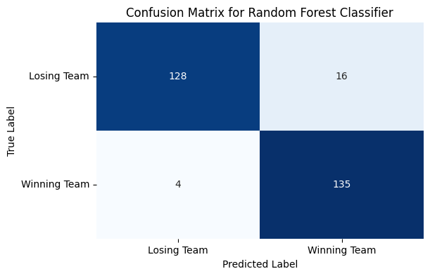
../../_images/bb419041bb3ececb7e07e2fb8fd650a618f1d1027264c425e497850f7500d7af.png

A classification report will sum up the confusion matrix with three metrics: precision, recall, and f1 score. According to https://medium.com/analytics-vidhya/evaluating-a-random-forest-model-9d165595ad56:

Precision is the number of correctly-identified members of a class divided by all the times the model predicted that class.
Recall is the number of members of a class that the classifier identified correctly divided by the total number of members in that class.
F1 score combines precision and recall into one metric. If precision and recall are both high, F1 will be high, too. If they are both low, F1 will be low. If one is high and the other low, F1 will be low.

print(classification_report(y_test, rfc_test_pred))

              precision    recall  f1-score   support

       False       0.97      0.89      0.93       144
        True       0.89      0.97      0.93       139

    accuracy                           0.93       283
   macro avg       0.93      0.93      0.93       283
weighted avg       0.93      0.93      0.93       283

Because the precision, recall, and f1 scores for both classes are high (\(\geq0.89\)), we can conclude that the random forest model is accurate at predicting whether a team has a winning record based on their stats. We can now analyze which stats were most important in determining a team’s success.

pd.Series(rfc.feature_importances_, index=rfc.feature_names_in_).sort_values(ascending=False)

runs_scored               0.192366
earned_run_average        0.134273
opponents_runs_scored     0.113034
earned_runs_allowed       0.091288
saves                     0.067500
hits                      0.064919
walks_allowed             0.048037
homeruns                  0.044631
hits_allowed              0.035169
walks                     0.033901
shutouts                  0.024170
outs_pitches              0.021774
doubles                   0.014424
at_bats                   0.014272
homeruns_allowed          0.012837
errors                    0.012371
sacrifice_flies           0.012179
strikeouts_by_batters     0.008981
fielding_percentage       0.008807
triples                   0.007699
strikeouts_by_pitchers    0.007344
complete_games            0.006878
caught_stealing           0.006677
stolen_bases              0.006267
batters_hit_by_pitch      0.005247
double_plays              0.004955
dtype: float64

runs_scored, opponents_runs_scored, and earned_run_average had the highest feature importances, which means that they were the most significant stats towards a team’s success. This agrees with the previous results found in the linear regression model, which found that earned_run_average had the greatest negative effect on winning percentage and runs_scored had one of the greatest positive effects on winning percentage.

Neural Network#

Another criteria to judge a team’s success is how far it goes in the playoffs. Now I will drop the rows with missing values in wild_card_winner.

df_playoffs = df_rate[~df_rate['wild_card_winner'].isna()]
df_playoffs.isna().sum(axis=0)

year                      0
games_played              0
wins                      0
losses                    0
division_winner           0
wild_card_winner          0
league_winner             0
world_series_winner       0
runs_scored               0
at_bats                   0
hits                      0
doubles                   0
triples                   0
homeruns                  0
walks                     0
strikeouts_by_batters     0
stolen_bases              0
caught_stealing           0
batters_hit_by_pitch      0
sacrifice_flies           0
opponents_runs_scored     0
earned_runs_allowed       0
earned_run_average        0
complete_games            0
shutouts                  0
saves                     0
outs_pitches              0
hits_allowed              0
homeruns_allowed          0
walks_allowed             0
strikeouts_by_pitchers    0
errors                    0
double_plays              0
fielding_percentage       0
win_percentage            0
is_win                    0
dtype: int64

I will create a new column in df_playoffs called playoffs that correlates to how far each team made in the playoffs. \(0\) correlates to no playoff series wins, \(1\) correlates to winning the wild card, \(2\) correlates to winning the league championship series, and \(3\) correlates to winning the world series. I created playoffs using code from: https://stackoverflow.com/questions/26886653/create-new-column-based-on-values-from-other-columns-apply-a-function-of-multi

conditions = [df_playoffs['world_series_winner'] == 'Y', df_playoffs['league_winner'] == 'Y', df_playoffs['wild_card_winner'] == 'Y']
outputs = [3, 2, 1]
df_playoffs['playoffs'] = np.select(conditions, outputs)
df_playoffs

/tmp/ipykernel_37/169299682.py:4: SettingWithCopyWarning: 
A value is trying to be set on a copy of a slice from a DataFrame.
Try using .loc[row_indexer,col_indexer] = value instead

See the caveats in the documentation: https://pandas.pydata.org/pandas-docs/stable/user_guide/indexing.html#returning-a-view-versus-a-copy
  df_playoffs['playoffs'] = np.select(conditions, outputs)

	year	games_played	wins	losses	division_winner	wild_card_winner	league_winner	world_series_winner	runs_scored	at_bats	...	hits_allowed	homeruns_allowed	walks_allowed	strikeouts_by_pitchers	errors	double_plays	fielding_percentage	win_percentage	is_win	playoffs
2010	1995	144	90	54	Y	N	Y	Y	0.539241	0.759990	...	0.594993	0.252830	0.455399	0.538106	0.446927	0.462428	0.608696	0.625000	True	3
2011	1995	144	71	73	N	N	N	N	0.613924	0.765699	...	0.581001	0.411321	0.591549	0.417244	0.290503	0.624277	0.782609	0.493056	False	0
2012	1995	144	86	58	Y	N	N	N	0.724051	0.805411	...	0.708395	0.328302	0.517997	0.384911	0.558659	0.682081	0.434783	0.597222	True	0
2013	1995	145	78	67	N	N	N	N	0.736709	0.810871	...	0.687776	0.464151	0.533646	0.394919	0.418994	0.502890	0.608696	0.537931	True	0
2014	1995	145	68	76	N	N	N	N	0.678481	0.821047	...	0.734904	0.467925	0.738654	0.387991	0.491620	0.566474	0.521739	0.468966	False	0
...	...	...	...	...	...	...	...	...	...	...	...	...	...	...	...	...	...	...	...	...	...
2779	2020	58	30	28	N	Y	N	N	0.026582	0.000000	...	0.000000	0.109434	0.092332	0.058507	0.072626	0.075145	0.652174	0.517241	True	1
2780	2020	60	40	20	Y	N	Y	N	0.088608	0.055349	...	0.072901	0.113208	0.035994	0.126251	0.072626	0.109827	0.739130	0.666667	True	2
2781	2020	60	22	38	N	N	N	N	0.006329	0.045669	...	0.075847	0.154717	0.142410	0.077752	0.111732	0.040462	0.565217	0.366667	False	0
2782	2020	60	32	28	N	Y	N	N	0.105063	0.067262	...	0.103829	0.154717	0.164319	0.100847	0.100559	0.080925	0.608696	0.533333	True	1
2783	2020	60	26	34	N	N	N	N	0.093671	0.053611	...	0.126657	0.203774	0.111111	0.092379	0.106145	0.086705	0.565217	0.433333	False	0

774 rows × 37 columns

Because the target variable is_win is categorical, the model will use each row’s stats to determine its class in playoffs, which is a classification problem. Therefore, I will try to use a neural network to model the relationship between stats and playoffs, using the code from https://www.tensorflow.org/tutorials/keras/classification. I also separated the data into training and testing data, which allow us to see if the neural network has overfit our data by testing the model on the testing data.

X_train, X_test, y_train, y_test = train_test_split(df_playoffs[cols], df_playoffs['playoffs'], test_size=0.2)

model = tf.keras.Sequential([
    tf.keras.layers.Dense(30, activation='relu'),
    tf.keras.layers.Dense(4)
])
model.compile(optimizer='adam',
              loss=tf.keras.losses.SparseCategoricalCrossentropy(from_logits=True),
              metrics=['accuracy'])
model.fit(X_train, y_train, epochs=10);

Epoch 1/10
20/20 [==============================] - 1s 5ms/step - loss: 0.9253 - accuracy: 0.8336
Epoch 2/10
20/20 [==============================] - 0s 5ms/step - loss: 0.6009 - accuracy: 0.8627
Epoch 3/10
20/20 [==============================] - 0s 5ms/step - loss: 0.5611 - accuracy: 0.8627
Epoch 4/10
20/20 [==============================] - 0s 5ms/step - loss: 0.5538 - accuracy: 0.8627
Epoch 5/10
20/20 [==============================] - 0s 1ms/step - loss: 0.5485 - accuracy: 0.8627
Epoch 6/10
20/20 [==============================] - 0s 2ms/step - loss: 0.5459 - accuracy: 0.8627
Epoch 7/10
20/20 [==============================] - 0s 2ms/step - loss: 0.5434 - accuracy: 0.8627
Epoch 8/10
20/20 [==============================] - 0s 5ms/step - loss: 0.5411 - accuracy: 0.8627
Epoch 9/10
20/20 [==============================] - 0s 4ms/step - loss: 0.5399 - accuracy: 0.8627
Epoch 10/10
20/20 [==============================] - 0s 5ms/step - loss: 0.5374 - accuracy: 0.8627

The model’s accuracy on the training data is \(0.8627\) (above), while the model’s accuracy on the testing data is \(0.8065\) (below).

test_loss, test_acc = model.evaluate(X_test,  y_test, verbose=2)
print('Test accuracy:', test_acc)

5/5 - 0s - loss: 0.6691 - accuracy: 0.8065 - 86ms/epoch - 17ms/step
Test accuracy: 0.8064516186714172

Now let’s look at the values predicted by the model.

probability_model = tf.keras.Sequential([model, 
                                         tf.keras.layers.Softmax()])
predictions = probability_model.predict(X_test)
lst = [np.argmax(row) for row in predictions]
np.unique(lst, return_counts=True)

5/5 [==============================] - 0s 2ms/step

(array([0]), array([155]))

This indicates that the model has predicted all teams in the testing data to belong to the \(0\) class of playoffs. Evidently, the neuron network was not able to distinguish a significant difference in the stats between teams that had playoff success and teams that did not. Therefore, none of the stats are statistically significant in determining a team’s playoff success.

Summary#

Using linear regression and a random forest, I determined that a MLB team’s success during the regular season can be predicted by some stats. In particular, runs scored and saves positively correlate to wins, while runs allowed and walks allowed negatively correlate to wins. However, there appears to be no correlation between any of the stats and a team’s playoff success, as shown by a neural network.

References#

Your code above should include references. Here is some additional space for references.

What is the source of your dataset(s)? https://www.retrosheet.org

List any other references that you found helpful.