Predicting Income Above a Threshold

Author: Timothy Cho

Course Project, UC Irvine, Math 10, F23

Introduction

We have one main goal in this section: given a set of people, and knowing a little bit about their work background (work, education, and number of hours per week), can we predict with high accuracy whether someone makes more than $50000 per year in income? Our first approach will be numerical, which is like what we did in Math 10. However, we will also explore the data using the categorical pieces we have, and we will learn how to do a classification problem, but the inputs are categorical rather than numerical.

Setting up the Data

In this section, we import the Adult dataset from the UC Irvine Machine Learning Repository and convert the data into our DataFrame df. Next, we clean out any missing values, so that our data will be ready for classification later.

We start by importing the necessary modules.

!pip install ucimlrepo

Requirement already satisfied: ucimlrepo in /root/venv/lib/python3.9/site-packages (0.0.3)

[notice] A new release of pip is available: 23.0.1 -> 23.3.1
[notice] To update, run: pip install --upgrade pip

import pandas as pd
import numpy as np
import altair as alt

Next, we load the data from the UCI repository and convert it to a DataFrame.

from ucimlrepo import fetch_ucirepo 
  
# fetch dataset 
adult = fetch_ucirepo(id=2)
# data (as pandas dataframes) 
X = adult.data.features 
y = adult.data.targets 

df = pd.DataFrame(data = X)
df['income'] = y
df.sample(20) # take a look at the data

	age	workclass	fnlwgt	education	education-num	marital-status	occupation	relationship	race	sex	capital-gain	capital-loss	hours-per-week	native-country	income
25956	32	Private	27207	10th	6	Never-married	Craft-repair	Not-in-family	White	Male	0	0	50	United-States	<=50K
20391	36	Local-gov	251091	Some-college	10	Married-civ-spouse	Protective-serv	Husband	White	Male	0	0	40	United-States	>50K
171	28	State-gov	175325	HS-grad	9	Married-civ-spouse	Protective-serv	Husband	White	Male	0	0	40	United-States	<=50K
33047	20	Private	273989	HS-grad	9	Never-married	Transport-moving	Own-child	White	Male	0	0	40	United-States	<=50K.
39628	36	Local-gov	254202	Prof-school	15	Divorced	Prof-specialty	Unmarried	White	Female	0	0	24	Germany	<=50K.
13797	30	Private	54929	HS-grad	9	Married-civ-spouse	Sales	Husband	White	Male	0	0	55	United-States	<=50K
46905	33	Private	133861	HS-grad	9	Married-civ-spouse	Craft-repair	Husband	White	Male	0	0	62	United-States	<=50K.
35796	21	Private	287681	HS-grad	9	Never-married	Machine-op-inspct	Own-child	White	Male	0	0	40	Mexico	<=50K.
905	46	Private	171550	HS-grad	9	Divorced	Machine-op-inspct	Not-in-family	White	Female	0	0	38	United-States	<=50K
12903	50	Private	209320	Bachelors	13	Married-civ-spouse	Sales	Husband	White	Male	0	0	40	United-States	>50K
13038	58	Private	214502	9th	5	Married-civ-spouse	Handlers-cleaners	Husband	White	Male	0	0	50	United-States	>50K
216	50	Private	313321	Assoc-acdm	12	Divorced	Sales	Not-in-family	White	Female	0	0	40	United-States	<=50K
28843	22	Private	218343	HS-grad	9	Never-married	Other-service	Own-child	White	Female	0	0	40	United-States	<=50K
37620	27	Private	315640	Masters	14	Never-married	Prof-specialty	Not-in-family	Asian-Pac-Islander	Male	0	0	20	China	<=50K.
26259	18	?	91670	Some-college	10	Never-married	?	Own-child	Asian-Pac-Islander	Female	0	0	40	United-States	<=50K
13299	44	Private	214838	HS-grad	9	Married-civ-spouse	Machine-op-inspct	Husband	White	Male	0	0	45	United-States	>50K
47874	27	Private	160291	Some-college	10	Never-married	Adm-clerical	Unmarried	Black	Female	0	0	40	Germany	<=50K.
21459	26	Private	113571	HS-grad	9	Never-married	Transport-moving	Not-in-family	White	Male	0	0	70	United-States	<=50K
35292	34	Self-emp-not-inc	264351	HS-grad	9	Married-civ-spouse	Farming-fishing	Husband	White	Male	0	0	40	Mexico	<=50K.
21063	64	State-gov	111795	Bachelors	13	Married-civ-spouse	Craft-repair	Husband	White	Male	0	0	45	United-States	>50K

Cleaning the Data

As we can see from the data sample above, our DataFrame df is quite messy, with a lot of categorical/nominal data, and very confusing categories, and with a lot of missing values. Additionally, the df['income'] column should be binary, but the way the data is encoded makes it an object. Our goal in this section is to clean up the data, so that clearly binary categories are stored with True/False values. We will also get rid of all rows with missing values.

df = df.dropna() # drops any row with a missing value

df.sample(10)

	age	workclass	fnlwgt	education	education-num	marital-status	occupation	relationship	race	sex	capital-gain	capital-loss	hours-per-week	native-country	income
15150	29	Private	213842	Some-college	10	Married-civ-spouse	Craft-repair	Husband	White	Male	0	0	40	United-States	<=50K
11767	38	State-gov	346766	HS-grad	9	Divorced	Adm-clerical	Unmarried	White	Female	0	0	40	United-States	<=50K
1551	17	Private	130806	10th	6	Never-married	Handlers-cleaners	Own-child	White	Male	0	0	24	United-States	<=50K
4052	31	Private	225053	HS-grad	9	Divorced	Transport-moving	Not-in-family	White	Male	0	0	45	United-States	<=50K
20249	80	Private	252466	Assoc-voc	11	Married-civ-spouse	Craft-repair	Husband	White	Male	0	0	24	United-States	<=50K
32027	46	Local-gov	140219	Masters	14	Divorced	Prof-specialty	Not-in-family	White	Female	8614	0	55	United-States	>50K
18858	53	Private	96062	Some-college	10	Married-civ-spouse	Exec-managerial	Husband	White	Male	0	1740	40	United-States	<=50K
36115	37	Private	108282	Bachelors	13	Married-civ-spouse	Exec-managerial	Husband	White	Male	0	0	45	United-States	<=50K.
5269	59	Private	43221	9th	5	Married-civ-spouse	Transport-moving	Husband	White	Male	0	0	60	United-States	>50K
19163	19	Private	170800	HS-grad	9	Never-married	Craft-repair	Own-child	White	Male	0	0	60	United-States	<=50K

The income column has the issue that <=50K and <=50K. represent the same value (and similarly with >50K and >50K.). We now convert this row into a True/False binary column.

income = df['income'].str.contains(">50K")
df['income>50k'] = income
df.sample(10)

	age	workclass	fnlwgt	education	education-num	marital-status	occupation	relationship	race	sex	capital-gain	capital-loss	hours-per-week	native-country	income	income>50k
31093	45	State-gov	144351	Masters	14	Married-civ-spouse	Prof-specialty	Husband	White	Male	0	0	40	United-States	>50K	True
14049	38	Private	117528	Bachelors	13	Never-married	Other-service	Other-relative	White	Female	0	0	45	United-States	<=50K	False
24214	20	Private	316043	11th	7	Never-married	Other-service	Own-child	Black	Male	594	0	20	United-States	<=50K	False
35309	24	Private	99697	HS-grad	9	Never-married	Handlers-cleaners	Own-child	White	Female	0	0	40	United-States	<=50K.	False
36406	55	Private	119344	HS-grad	9	Married-civ-spouse	Prof-specialty	Own-child	White	Female	0	0	40	United-States	<=50K.	False
15892	90	Private	88991	Bachelors	13	Married-civ-spouse	Exec-managerial	Wife	White	Female	0	0	40	England	>50K	True
15279	52	Self-emp-inc	334273	Doctorate	16	Married-civ-spouse	Prof-specialty	Husband	White	Male	99999	0	65	United-States	>50K	True
23945	21	Private	163333	Some-college	10	Never-married	Other-service	Own-child	White	Female	0	0	35	United-States	<=50K	False
18463	74	Private	188709	Prof-school	15	Married-civ-spouse	Prof-specialty	Husband	White	Male	99999	0	50	United-States	>50K	True
13845	65	?	105017	Bachelors	13	Married-civ-spouse	?	Husband	White	Male	0	0	40	United-States	<=50K	False

The old df['income'] row is useless now, so we drop it from our DataFrame.

df = df.drop('income', axis=1)

df

	age	workclass	fnlwgt	education	education-num	marital-status	occupation	relationship	race	sex	capital-gain	capital-loss	hours-per-week	native-country	income>50k
0	39	State-gov	77516	Bachelors	13	Never-married	Adm-clerical	Not-in-family	White	Male	2174	0	40	United-States	False
1	50	Self-emp-not-inc	83311	Bachelors	13	Married-civ-spouse	Exec-managerial	Husband	White	Male	0	0	13	United-States	False
2	38	Private	215646	HS-grad	9	Divorced	Handlers-cleaners	Not-in-family	White	Male	0	0	40	United-States	False
3	53	Private	234721	11th	7	Married-civ-spouse	Handlers-cleaners	Husband	Black	Male	0	0	40	United-States	False
4	28	Private	338409	Bachelors	13	Married-civ-spouse	Prof-specialty	Wife	Black	Female	0	0	40	Cuba	False
...	...	...	...	...	...	...	...	...	...	...	...	...	...	...	...
48836	33	Private	245211	Bachelors	13	Never-married	Prof-specialty	Own-child	White	Male	0	0	40	United-States	False
48837	39	Private	215419	Bachelors	13	Divorced	Prof-specialty	Not-in-family	White	Female	0	0	36	United-States	False
48839	38	Private	374983	Bachelors	13	Married-civ-spouse	Prof-specialty	Husband	White	Male	0	0	50	United-States	False
48840	44	Private	83891	Bachelors	13	Divorced	Adm-clerical	Own-child	Asian-Pac-Islander	Male	5455	0	40	United-States	False
48841	35	Self-emp-inc	182148	Bachelors	13	Married-civ-spouse	Exec-managerial	Husband	White	Male	0	0	60	United-States	True

47621 rows × 15 columns

Next, the sex trait is binary here, so we change that into a True/False column.

sex = df['sex'].str.contains('Male')
sex
df['is-male'] = sex
df = df.drop('sex', axis=1)

df.sample(10)

	age	workclass	fnlwgt	education	education-num	marital-status	occupation	relationship	race	capital-gain	capital-loss	hours-per-week	native-country	income>50k	is-male
3275	58	Private	241056	Some-college	10	Divorced	Adm-clerical	Unmarried	White	0	0	46	United-States	False	False
22806	46	Private	403911	Assoc-voc	11	Married-civ-spouse	Craft-repair	Husband	Black	0	0	40	United-States	True	True
19170	52	State-gov	314627	Masters	14	Divorced	Prof-specialty	Not-in-family	Asian-Pac-Islander	0	0	40	United-States	False	False
23728	44	Private	152150	Assoc-acdm	12	Separated	Exec-managerial	Not-in-family	White	0	0	40	United-States	False	True
24312	20	State-gov	147280	HS-grad	9	Never-married	Other-service	Other-relative	Other	0	0	40	United-States	False	True
9352	41	State-gov	116520	Doctorate	16	Married-civ-spouse	Prof-specialty	Husband	White	0	0	40	United-States	True	True
19123	20	Private	62865	HS-grad	9	Never-married	Priv-house-serv	Not-in-family	White	0	0	45	United-States	False	False
19610	22	Private	340543	HS-grad	9	Never-married	Tech-support	Not-in-family	White	0	0	40	United-States	False	False
35840	19	Private	382688	10th	6	Never-married	Handlers-cleaners	Not-in-family	White	0	0	20	United-States	False	True
38961	57	Private	157271	11th	7	Divorced	Other-service	Not-in-family	Black	0	0	54	United-States	False	True

Now, our data is ready to be analyzed.

Time Investment versus Income: Logistic Regression

In this section, we examine if a person’s education level and the number of hours they work determine whether they make more than $50000 a year. This is just a regular binary classification problem like we have been doing in Math 10; we will later use the categorical data to make classifications, and we will see new things when we get there.

Intuitively, we should expect that the more hours worked and the higher the education level, the person’s income is more likely to be above $50000. That is, the more time they take to do things like educate themselves/go to work, the higher we expcet their income to be. Let us see if this is actually the case.

Visualizing the Data

Unfortunately, our dataset is far too large for Deepnote to render output. To remedy this, we will plot a few different plots by randomly taking 500 samples 5 times.

cols = ['education-num', 'hours-per-week'] # these are the columns we are interested in
rng = np.random.default_rng(seed=63)
seed_list = [rng.integers(1, 10**6) for i in range(5)]

n = 500
circ_size = 60
chart_list = []
# generate our 5 randomized charts
for s in seed_list:
    chart_list.append(alt.Chart(df.sample(n, random_state=s)).mark_circle(size=circ_size).encode(
        x = cols[0],
        y = cols[1],
        color = 'income>50k:N'
        ).properties(title=f'Education Level/Hours per Week, 500 samples, seed={s}'))

alt.hconcat(*chart_list)

As we can see, there seems to be a slight correlation between the education-num and the income: we see more orange points towards the right of the chart. On the other had, the number of hours worked per week does not seem to affect whether someone makes more than $50000. Now, let us implement logistic regression to see the exact correlations.

Analysis

We now fit our data to the logistic regression model. We will let 90% of the data be training data, and the remaining 10% be testing data.

from sklearn.linear_model import LogisticRegression
from sklearn.model_selection import train_test_split

clf = LogisticRegression()
X_train, X_test, y_train, y_test = train_test_split(df[cols], df['income>50k'], test_size=0.1, random_state=63)
clf.fit(X_train, y_train)

LogisticRegression()

In a Jupyter environment, please rerun this cell to show the HTML representation or trust the notebook.
On GitHub, the HTML representation is unable to render, please try loading this page with nbviewer.org.

Let us see some information about what we got for clf. Remember that we set cols = ['education-num', 'hours-per-week'].

clf.classes_

array([False,  True])

clf.coef_

array([[0.34405795, 0.0401318 ]])

clf.intercept_

array([-6.49326522])

The above tells us that if \(x_1\) is the education level, and \(x_2\) is the number of hours worked per week, the probability that someone gets paid over $50000 a month is given approximately by the function $\(f(x_1, x_2) =\displaystyle \frac 1{1+\exp(-0.339x_1 - 0.040x_2 + 6.428)}\)$. Now, let us see how well our model performs on the test data.

clf.score(X_test, y_test)

0.7772412345160613

The performance of our model is not bad, but also not great: we might be overfitting slightly, and the correlation was not as strong as what we might have intuitively expected. Looking back to the charts we made, it seemed as if the number of hours worked barely had an effect on the income. What if we tried removing the number of hours column and running regression again?

clf2 = LogisticRegression()
X_train, X_test, y_train, y_test = train_test_split(df[['education-num']], df['income>50k'], test_size=0.1, random_state=63)
clf2.fit(X_train, y_train)

LogisticRegression()

In a Jupyter environment, please rerun this cell to show the HTML representation or trust the notebook.
On GitHub, the HTML representation is unable to render, please try loading this page with nbviewer.org.

For this new model, we see that the coefficient for the education level is still around 0.35:

clf2.coef_

array([[0.36081249]])

clf2.intercept_

array([-4.97816245])

How well does this perform on the test set?

clf2.score(X_test, y_test)

0.7753516691161033

This was around the same as when we had the number of hours worked. Hence, there might be a correlation between education level and a person’s income, but this correlation seems a lot weaker than we expected. What if we approach this dataset using the categorical data instead?

Types of Education versus Income: A Categorical Approach

In the last section, we saw that when we plugged in the education level of a person (education-num), our models were able to predict with around 77% accuracy whether a person made more than $50000 a year. This is much better than random guessing, but 77% accuracy does not suggest a very strong correlation. However, one thing that the education-num column leaves out is the type of school the person went to: for example, we would expect a PhD to have different job opportunities than someone who went to a professional training school; however, this information is completely missing from the numeric data we were provided. What if we can get a stronger correlation using the categorical education column instead?

Of course, we cannot use logistic regression here, as our inputs are nominal data. Additionally, we have a second problem, as the standard DecisionTreeClassifier we learned in Math 10, which we plan to use, does not normally accept categorical data, so we cannot directly fit the education column into clf. Instead, we use the pandas method get_dummies to convert our education data into a set of binary variables, so that the DecisionTreeClassifier could properly process them. This technique is known as one-hot encoding.

from sklearn.tree import DecisionTreeClassifier

Making Our Data Understandable to DecisionTreeClassifier: One-Hot Encoding

In the code below, we one-hot encode our education data. Notice that each unique entry in the education column becomes its own column in the DataFrame below, and each 1 corresponds to what the original category was in the original DataFrame.

encoded = pd.get_dummies(df['education'])
encoded

	10th	11th	12th	1st-4th	5th-6th	7th-8th	9th	Assoc-acdm	Assoc-voc	Bachelors	Doctorate	HS-grad	Masters	Preschool	Prof-school	Some-college
0	0	0	0	0	0	0	0	0	0	1	0	0	0	0	0	0
1	0	0	0	0	0	0	0	0	0	1	0	0	0	0	0	0
2	0	0	0	0	0	0	0	0	0	0	0	1	0	0	0	0
3	0	1	0	0	0	0	0	0	0	0	0	0	0	0	0	0
4	0	0	0	0	0	0	0	0	0	1	0	0	0	0	0	0
...	...	...	...	...	...	...	...	...	...	...	...	...	...	...	...	...
48836	0	0	0	0	0	0	0	0	0	1	0	0	0	0	0	0
48837	0	0	0	0	0	0	0	0	0	1	0	0	0	0	0	0
48839	0	0	0	0	0	0	0	0	0	1	0	0	0	0	0	0
48840	0	0	0	0	0	0	0	0	0	1	0	0	0	0	0	0
48841	0	0	0	0	0	0	0	0	0	1	0	0	0	0	0	0

47621 rows × 16 columns

Analysis

Now, our data is ready to be analyzed. There is one slight technicality that we need to be careful with: notice that that encoded from above is a DataFrame in its own right, so our source data should be drawn from encoded, but our prediction target is in the column df['income>50k']. We will set the max_depth of our classifier clf to be 4 to prevent overfitting.

clf3 = DecisionTreeClassifier(max_depth=4)
X_train, X_test, y_train, y_test = train_test_split(encoded, df['income>50k'], test_size=0.1, random_state=60)

clf3.fit(X_train, y_train)

DecisionTreeClassifier(max_depth=4)

In a Jupyter environment, please rerun this cell to show the HTML representation or trust the notebook.
On GitHub, the HTML representation is unable to render, please try loading this page with nbviewer.org.

Let us visualize how our classifier makes decisions below. We will actually write a function for this, as we will be repeating the same code a lot later on. The code below for plotting the decision tree was taken from the class notes.

import matplotlib.pyplot as plt
from sklearn.tree import plot_tree
# function to visualize decision tree
def plot(classifier):
    classes = [str(cls) for cls in classifier.classes_]
    plot_tree(classifier, 
                feature_names=classifier.feature_names_in_,
                class_names=classes,
                filled=True)

plot(clf3)

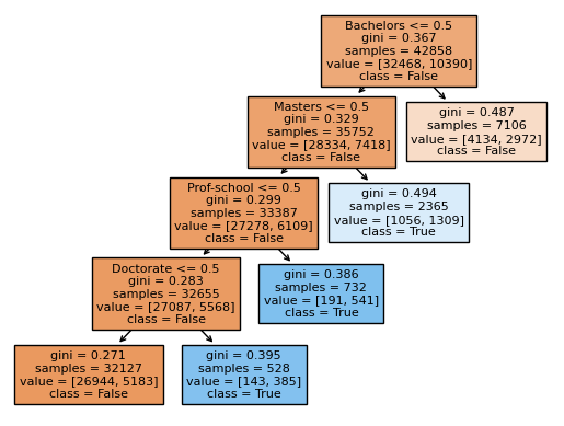
We should remember that each category in the education column is mutually exclusive. Hence, this means that the decision tree’s decisions seem logical to us: the tree first checks if the person’s highest education level is a Bachelor’s. If this is probably not the case, then the tree checks for higher and higher degrees, until the Doctorate. Then, if they tree thinks that the person does not hold any of the degrees it checks, it renders a False decision.

Now, let us check its accuracy on the test set.

clf3.score(X_test, y_test)

0.7751417174049968

This accuracy is almost the same as when we did the logistic regression. Hence, we see that no matter if we do things categorically or numerically, in this area of education, we were able to predict with around 77% accuracy whether a person made more than $50000 a year. Hence, we are confident in saying that there is a slight correlation between education and income. We also see a curiosity: the accuracy scores between our decision tree and our logistic classifier were equal up to the third decimal place. It seems like the decision tree behaved a lot like the logistic classifier in this case.

Does the Job Worked Affect Income?

In this short section, we apply our techniques from the previous section to see if it is really true that the type of job that you work determines the amount of money you might make.

Preparing Our Data

As before, we need to one-hot encode our data in order to use DecisionTreeClassifier.

encoded = pd.get_dummies(df['occupation'])
encoded

	?	Adm-clerical	Armed-Forces	Craft-repair	Exec-managerial	Farming-fishing	Handlers-cleaners	Machine-op-inspct	Other-service	Priv-house-serv	Prof-specialty	Protective-serv	Sales	Tech-support	Transport-moving
0	0	1	0	0	0	0	0	0	0	0	0	0	0	0	0
1	0	0	0	0	1	0	0	0	0	0	0	0	0	0	0
2	0	0	0	0	0	0	1	0	0	0	0	0	0	0	0
3	0	0	0	0	0	0	1	0	0	0	0	0	0	0	0
4	0	0	0	0	0	0	0	0	0	0	1	0	0	0	0
...	...	...	...	...	...	...	...	...	...	...	...	...	...	...	...
48836	0	0	0	0	0	0	0	0	0	0	1	0	0	0	0
48837	0	0	0	0	0	0	0	0	0	0	1	0	0	0	0
48839	0	0	0	0	0	0	0	0	0	0	1	0	0	0	0
48840	0	1	0	0	0	0	0	0	0	0	0	0	0	0	0
48841	0	0	0	0	1	0	0	0	0	0	0	0	0	0	0

47621 rows × 15 columns

We have a slight issue here: one of the columns in our one-hot encoded data is labeled ?, which does not seem to be particularly useful to what we are doing. Hence, we are justified in dropping that column, which cleans the data.

encoded = encoded.drop("?", axis=1)

Now, our data is ready for analysis.

Analysis

We do the same steps as we did in the previous section.

clf4 = DecisionTreeClassifier(max_depth=6)
X_train, X_test, y_train, y_test = train_test_split(encoded, df['income>50k'], test_size=0.1, random_state=57)
clf4.fit(X_train, y_train)

DecisionTreeClassifier(max_depth=6)

In a Jupyter environment, please rerun this cell to show the HTML representation or trust the notebook.
On GitHub, the HTML representation is unable to render, please try loading this page with nbviewer.org.

Let us take a look at how the decisions were made.

plot(clf4)

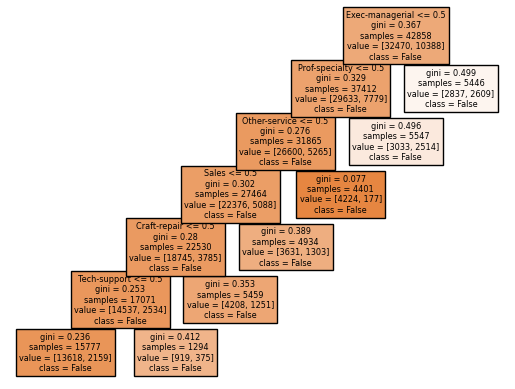
Immediately, we should see that something is off about the way decisions are being made: the machine renders a False decision for every job. This suggests to us that occupation is not a great way to determine someone’s income, at least for the jobs mentioned here. However, there are still patterns: the machine is less sure about its False decision when the probablity of being in a executive/managerial or a professional/specialty position is at least 0.5, which kind of makes sense. Let us see the classifier’s score on the test data.

clf4.score(X_test, y_test)

0.7579256770942683

Surprisingly, the machine does a lot better when it assigns False decisions to everyone when compared to randomly guessing with 50% probability of being correct. However, the correlation between job type and income still seems to be slight, rather than actually predictable.

Conclusion

In this dataset, we saw two factors that have some impact on the income: the job worked and the education level. However, the correlation we got seemed to be sort of weak in both cases: our accuracy on the test data was around 75% to 77%, which is better than making a 50/50 guess at whether someone makes more than $50000 a year, but still not great in comparison to some of the examples we saw in class. However, we still expect there to be a correlation. If we had a dataset that gave the income as a numeric value, we would expect a regression model to have higher accuracy, as the accuracy of that is judged by mean squared error instead. Hence, our conclusion is that while classification does seem to work out okay here, this problem is much better addressed by a regression model, where we predict the income directly instead of determining whether it passes a certain threshold.

References

Your code above should include references. Here is some additional space for references.

• What is the source of your dataset(s)? UCI ML Repository

• List any other references that you found helpful. Class notes; all other sources are linked above.