Transcation Fraud Detection

Transcation Fraud Detection#

Author: Xinyu Chen

Course Project, UC Irvine, Math 10, F23

Introduction#

This project predicts the fraud detection using features. However, there also exists no-use features, so I have to find which dedicates most to the prediction. Also, it has results of 0 and 1, which presents to be a supervised learning and binary classification problem.

1. import data#

This original dataset costs long time to process, you may switch directly to the second dataset to run the cell, it will take shorter time, this section is for simplify the dataset. You can see the instruction underneath to straightforwardly run the second csv file.#

#It will take up to 20-25 sec to execute the csv.
import pandas as pd
df=pd.read_csv("/work/PS_20174392719_1491204439457_log.csv").copy()
df.head(5)

	step	type	amount	nameOrig	oldbalanceOrg	newbalanceOrig	nameDest	oldbalanceDest	isFraud
0	1	PAYMENT	9839.64	C1231006815	170136.0	160296.36	M1979787155	0.0	0
1	1	PAYMENT	1864.28	C1666544295	21249.0	19384.72	M2044282225	0.0	0
2	1	TRANSFER	181.00	C1305486145	181.0	0.00	C553264065	0.0	1
3	1	CASH_OUT	181.00	C840083671	181.0	0.00	C38997010	21182.0	1
4	1	PAYMENT	11668.14	C2048537720	41554.0	29885.86	M1230701703	0.0	0

df.shape

(6362620, 11)

df.info()

<class 'pandas.core.frame.DataFrame'>
RangeIndex: 6362620 entries, 0 to 6362619
Data columns (total 11 columns):
 #   Column          Dtype  
---  ------          -----  
 0   step            int64  
 1   type            object 
 2   amount          float64
 3   nameOrig        object 
 4   oldbalanceOrg   float64
 5   newbalanceOrig  float64
 6   nameDest        object 
 7   oldbalanceDest  float64
 8   newbalanceDest  float64
 9   isFraud         int64  
 10  isFlaggedFraud  int64  
dtypes: float64(5), int64(3), object(3)
memory usage: 534.0+ MB

import warnings
warnings.filterwarnings('ignore',category = DeprecationWarning)

print("Number of duplicate rows:", df.duplicated().sum())

Number of duplicate rows: 0

There is no duplicated rows.

2.EDA#

What does each variable means? step
Transcation happens in a hour, no use
type
transaction type, sentence the affliation of the fraud
amount amount of the transcation
nameOrig the account payer
oldbalanceOrg the payer’s amount before the transcation
newbalanceOrig the payer’s amount after the transcation
nameDest the payee’s name
oldbalanceDest the payee’s amount before the transcation
newbalanceDest the payee’s amount after the transcation
isFraud Whether the transcation is a fraud(0,1), so it’s a supervised learning question
isFlaggedFraud Whether a transfer amount>200000, no big use now

We need to classify the fraud type because maybe not every type has the fraud record

grouped_counts = df[df['isFraud']==1].groupby('type').size()
grouped_counts

type
CASH_OUT    4116
TRANSFER    4097
dtype: int64

We can see that only ‘cash_out’ and ‘transfer’ type has the fraud record, so we can focus on these two. Also, considering the record and the fraud amount, there aren’t many fraud happens. Therefore, the x should only be data that contains ‘transfer’ and ‘cash_out’.

Therefore, we will only focus on data containing this two types. Also, since step only contains number 1, so we can drop it.

tmp = df.loc[(df['type'].isin(['TRANSFER', 'CASH_OUT'])),:]
for column in ['step']:
    if column in tmp.columns:
        tmp.drop(['step'], axis=1,inplace=True)
tmp.to_csv('first_processing_data.csv')

/shared-libs/python3.9/py/lib/python3.9/site-packages/pandas/core/frame.py:4308: SettingWithCopyWarning: 
A value is trying to be set on a copy of a slice from a DataFrame

See the caveats in the documentation: https://pandas.pydata.org/pandas-docs/stable/user_guide/indexing.html#returning-a-view-versus-a-copy
  return super().drop(

tmp.columns

Index(['type', 'amount', 'nameOrig', 'oldbalanceOrg', 'newbalanceOrig',
       'nameDest', 'oldbalanceDest', 'newbalanceDest', 'isFraud',
       'isFlaggedFraud'],
      dtype='object')

tmp.shape

(2770409, 10)

If the dataset provides too much time to process, it’s also fine to start the notebook from here.#

import pandas as pd
df=pd.read_csv('first_processing_data.csv').copy()
if df.columns[0] != 'type':
    df.drop(df.columns[0], axis=1, inplace=True)
print(df.shape)
#This will greatly decreases the processing time.
df.columns

(2770409, 10)

Index(['type', 'amount', 'nameOrig', 'oldbalanceOrg', 'newbalanceOrig',
       'nameDest', 'oldbalanceDest', 'newbalanceDest', 'isFraud',
       'isFlaggedFraud'],
      dtype='object')

df.sample(5)

	type	amount	nameOrig	oldbalanceOrg	nameDest	oldbalanceDest	newbalanceDest
2056112	CASH_OUT	84059.52	C1583877681	0.0	C1503134106	220619.67	304679.18
983956	CASH_OUT	40584.70	C1384648531	17215.0	C940141589	0.00	40584.70
2359232	CASH_OUT	310984.43	C893666197	0.0	C1618024942	481055.93	792040.36
923004	CASH_OUT	26021.74	C192862021	0.0	C2043549610	1618256.14	1644277.88
1286308	TRANSFER	1079362.35	C709778027	0.0	C446002180	2584452.81	4085189.07

Firstly, we need to decide whether to drop the isFlaggedFraud, an easy way to determine is that it contains only the transfer type, as the variable definition says, is not enough to decide whether an transcation is fraud, because there remains cash_out type, but we can look closer to it.

df[df.isFlaggedFraud == 1]

	type	amount	nameOrig	oldbalanceOrg	newbalanceOrig	nameDest	isFraud	isFlaggedFraud
1204984	TRANSFER	4953893.08	C728984460	4953893.08	4953893.08	C639921569	1	1
1422214	TRANSFER	1343002.08	C1100582606	1343002.08	1343002.08	C1147517658	1	1
1646619	TRANSFER	536624.41	C1035541766	536624.41	536624.41	C1100697970	1	1
2428454	TRANSFER	4892193.09	C908544136	4892193.09	4892193.09	C891140444	1	1
2619154	TRANSFER	10000000.00	C689608084	19585040.37	19585040.37	C1392803603	1	1
2619156	TRANSFER	9585040.37	C452586515	19585040.37	19585040.37	C1109166882	1	1
2688696	TRANSFER	3576297.10	C193696150	3576297.10	3576297.10	C484597480	1	1
2703826	TRANSFER	353874.22	C1684585475	353874.22	353874.22	C1770418982	1	1
2729568	TRANSFER	2542664.27	C786455622	2542664.27	2542664.27	C661958277	1	1
2736011	TRANSFER	10000000.00	C19004745	10399045.08	10399045.08	C1806199534	1	1
2736013	TRANSFER	399045.08	C724693370	10399045.08	10399045.08	C1909486199	1	1
2741701	TRANSFER	3441041.46	C917414431	3441041.46	3441041.46	C1082139865	1	1
2765218	TRANSFER	3171085.59	C1892216157	3171085.59	3171085.59	C1308068787	1	1
2770249	TRANSFER	10000000.00	C2140038573	17316255.05	17316255.05	C1395467927	1	1
2770251	TRANSFER	7316255.05	C1869569059	17316255.05	17316255.05	C1861208726	1	1
2770373	TRANSFER	5674547.89	C992223106	5674547.89	5674547.89	C1366804249	1	1

We can also validate the variable by using the random forest to decide the importance of each variable.

import pandas as pd
import numpy as np
from sklearn.ensemble import RandomForestClassifier

df_test1=df.copy()
X = df_test1.drop(['isFraud','type','nameOrig','nameDest'], axis=1)  # 特征列
y = df_test1['isFraud']  # 目标列

num_samples = 20

feature_importance_scores = []

for i in range(num_samples):
    sample_indices = np.random.choice(len(X), size=5000, replace=False)
    X_sample = X.iloc[sample_indices]
    y_sample = y.iloc[sample_indices]
    
    rfc = RandomForestClassifier(n_estimators=100, random_state=42)
    rfc.fit(X_sample, y_sample)
    
    feature_importance_scores.append(rfc.feature_importances_)

average_feature_importance = np.mean(feature_importance_scores, axis=0)

feature_importance_dict = dict(zip(X.columns, average_feature_importance))

for feature, importance in feature_importance_dict.items():
    print(f"Feature: {feature}, Importance: {importance:.4f}")

Feature: amount, Importance: 0.1838
Feature: oldbalanceOrg, Importance: 0.3878
Feature: newbalanceOrig, Importance: 0.0454
Feature: oldbalanceDest, Importance: 0.1527
Feature: newbalanceDest, Importance: 0.2294
Feature: isFlaggedFraud, Importance: 0.0008

We can see that ithas very low importance, so we’d better drop it.

There is only 16 transcations this varible can know. If “isFlaggedFraud”=1, it’s definitly “isFraud”=1, but there remains fraud but the “isFlaggedFraud” doesn’t recognize. Therefore, the transcation doesn’t seem to have a good reflection of the label itself, so we’d better drop it.

df[(df.type=='TRANSFER') & ((df.amount >=2000000) | (abs(df.oldbalanceOrg-df.newbalanceOrig)>2000000) | (abs(df.newbalanceDest-df.oldbalanceDest)>2000000))]

	type	amount	nameOrig	oldbalanceOrg	newbalanceOrig	nameDest	oldbalanceDest	newbalanceDest	isFraud	isFlaggedFraud
4	TRANSFER	311685.89	C1984094095	10835.00	0.00	C932583850	6267.00	2719172.89	0	0
19	TRANSFER	125872.53	C1443967876	0.00	0.00	C392292416	348512.00	3420103.09	0	0
20	TRANSFER	379856.23	C1449772539	0.00	0.00	C1590550415	900180.00	19169204.93	0	0
21	TRANSFER	1505626.01	C926859124	0.00	0.00	C665576141	29031.00	5515763.34	0	0
24	TRANSFER	761507.39	C412788346	0.00	0.00	C1590550415	1280036.23	19169204.93	0	0
...	...	...	...	...	...	...	...	...	...	...
2770369	TRANSFER	10000000.00	C88849251	25674547.89	15674547.89	C1939028448	0.00	0.00	1	0
2770371	TRANSFER	10000000.00	C1945606464	15674547.89	5674547.89	C625944676	0.00	0.00	1	0
2770373	TRANSFER	5674547.89	C992223106	5674547.89	5674547.89	C1366804249	0.00	0.00	1	1
2770387	TRANSFER	4009058.39	C1044665079	4009058.39	0.00	C750074708	0.00	0.00	1	0
2770405	TRANSFER	6311409.28	C1529008245	6311409.28	0.00	C1881841831	0.00	0.00	1	0

47141 rows × 10 columns

The final decision whether to drop this variable is that it can’t filter all the transfer one that are >2000000, so I really don’t know what’s this varible for, so I will drop it. Also, I’ve figured out we can’t see through whether a transcation is fraud by calculating the spread of the old balanceOrg and new balanceorig or by the payee side or the amount side to decide in this question, to certify my conclusion, I will write the code.

df[(df.isFraud==0)&(df.type=='TRANSFER')&((df.amount!=(df.oldbalanceOrg-df.newbalanceOrig))|(df.amount!=abs(df.oldbalanceDest-df.newbalanceDest))|(abs(df.oldbalanceDest-df.newbalanceDest)!=abs(df.newbalanceDest-df.oldbalanceDest))|(df.oldbalanceDest-df.newbalanceDest+df.newbalanceDest-df.oldbalanceDest!=0))]

	type	amount	nameOrig	oldbalanceOrg	newbalanceOrig	nameDest	oldbalanceDest	newbalanceDest	isFraud	isFlaggedFraud
3	TRANSFER	215310.30	C1670993182	705.00	0.00	C1100439041	22425.00	0.00	0	0
4	TRANSFER	311685.89	C1984094095	10835.00	0.00	C932583850	6267.00	2719172.89	0	0
9	TRANSFER	62610.80	C1976401987	79114.00	16503.20	C1937962514	517.00	8383.29	0	0
14	TRANSFER	42712.39	C283039401	10363.39	0.00	C1330106945	57901.66	24044.18	0	0
15	TRANSFER	77957.68	C207471778	0.00	0.00	C1761291320	94900.00	22233.65	0	0
...	...	...	...	...	...	...	...	...	...	...
2770096	TRANSFER	92746.73	C587921214	5051.00	0.00	C930436926	279931.86	372678.59	0	0
2770097	TRANSFER	76507.70	C1157171835	13161.00	0.00	C720176528	274281.30	350789.00	0	0
2770098	TRANSFER	14563.03	C936960472	20705.00	6141.97	C1924752944	153878.31	168441.35	0	0
2770102	TRANSFER	139144.25	C1264043726	7075.00	0.00	C2093369248	49040158.93	49179303.19	0	0
2770112	TRANSFER	82096.45	C614459560	13492.00	0.00	C855350324	0.00	82096.45	0	0

524910 rows × 10 columns

We can’t simply treat it as a accounting problem, there usually exists other questions. Also, the condition of condition, old and new balanceorg can be treated as one feature by using +/-.

So what about the name of payer and payee? It’s rather a good point as we may need to think about before dropping it not to treat it as a feature. We can classify the data using C and M.

import numpy as np
df['type2'] = np.nan
df.loc[df.nameOrig.str.contains('C') & df.nameDest.str.contains('C'), 'type2'] = 'CC'
df.loc[df.nameOrig.str.contains('C') & df.nameDest.str.contains('M'), 'type2'] = 'CM'
df.loc[df.nameOrig.str.contains('M') & df.nameDest.str.contains('C'), 'type2'] = 'MC'
df.loc[df.nameOrig.str.contains('M') & df.nameDest.str.contains('C'), 'type2'] = 'MM'

df['type2'].value_counts()

CC    2770409
Name: type2, dtype: int64

Tricky part is that all fraud are CC in transfer and check out fraction, so it’s better throw them.

columns_to_drop = ['type2', 'nameOrig', 'nameDest', 'isFlaggedFraud']
df.drop(columns=[col for col in columns_to_drop if col in df.columns], inplace=True)

3.data cleaning and feature engineering#

Firstly, we need to change some column names to achieve the standardize effect.

df.rename(columns={'oldbalanceOrg': 'from_oldb', 'newbalanceOrig': 'from_newb','oldbalanceDest': 'to_oldb','newbalanceDest': 'to_newb'}, inplace=True)

Also, since I’ve only contained cash_out and transfer type as the only two columns that isFraud=1, the df columns can be set as the dataset. isFraud column should be set as Y for upcoming machine learning dataset setting.

Set the type of transcation into digital numbers for better classification.

df.loc[df.type=='TRANSFER','type'] = 0
df.loc[df.type=='CASH_OUT','type'] = 1

Next, we need to deal with the missing values. I’ve discussed before on whether to retain the ‘isFlaggedFraud’ variable when I find that from and to account has amount balance but ‘amount’ column remains 0 but not be considered as a fraud, and that may be a missing value problem. Here are two situations: one is that amount>0, but from_oldb=0 and from_newb=0, another situation is that amount>0, but to_oldb and to_newb=0.Thereforem we should examine the fraud amount to decide what we should do about it.

len(df.loc[(df.isFraud==1) & (df.from_oldb==0)& (df.from_newb==0)& (df.amount!=0)])/len(df[df['isFraud']==1])

0.0030439547059539756

len(df.loc[(df.isFraud==0) & (df.from_oldb==0)& (df.from_newb==0)& (df.amount!=0)])/len(df[df['isFraud']==0])

0.4737321319703598

It does have smaller probability that both are 0 is considered to be a fraud, therefore, we should set it still because it won’t influence much about the result of the fraud rate, we can treat it as nan to decrease the probability of wrongly treatment.

len(df.loc[(df.isFraud==1) & (df.to_oldb==0)& (df.to_newb==0)& (df.amount!=0)])/len(df[df['isFraud']==1])

0.4955558261293072

len(df.loc[(df.isFraud==0) & (df.to_oldb==0)& (df.to_newb==0)& (df.amount!=0)])/len(df[df['isFraud']==0])

0.0006176245277308345

The non fraud rate of the second situation has a low rate, we can tell that if to_b=0, it is more likely to be a fraud transcation, so we’d better change the number from 0 to -1 for the better usuage of the upcoming machine learning method.

df.loc[(df.to_oldb==0)& (df.to_newb==0)& (df.amount!=0),['to_oldb','to_newb']]=-1
df.loc[(df.from_oldb==0)& (df.from_newb==0)& (df.amount!=0),['from_oldb','from_newb']]=np.nan

To simplify the dataset, we won’t discuss any rows containing nan because it may increase unecessary burden to the model fitting in the next part.

df=df.dropna()

From the above missing value disscussion we cen tell that to_b and from_b has close relationship with amount, so we should set these three into a new variable since they prove to be similar function, let alone they point out to decrease missing value influence after combining together.

df['errorto_b']=df.to_newb+df.amount-df.to_oldb
df['errorfrom_b']=df.from_newb+df.amount-df.from_oldb

df.columns

Index(['type', 'amount', 'from_oldb', 'from_newb', 'to_oldb', 'to_newb',
       'isFraud', 'errorto_b', 'errorfrom_b'],
      dtype='object')

Before modeling, let’s evaluate again the feature importance.

import pandas as pd
import numpy as np
from sklearn.ensemble import RandomForestClassifier

df_test=df.copy()
X = df_test.drop('isFraud', axis=1)  
y = df_test['isFraud']  

num_samples = 20

feature_importance_scores = []

for i in range(num_samples):
    sample_indices = np.random.choice(len(X), size=5000, replace=False)
    X_sample = X.iloc[sample_indices]
    y_sample = y.iloc[sample_indices]
    
    rfc = RandomForestClassifier(n_estimators=100, random_state=42)
    rfc.fit(X_sample, y_sample)
    
    feature_importance_scores.append(rfc.feature_importances_)

average_feature_importance = np.mean(feature_importance_scores, axis=0)

feature_importance_dict = dict(zip(X.columns, average_feature_importance))

for feature, importance in feature_importance_dict.items():
    print(f"Feature: {feature}, Importance: {importance:.4f}")

Feature: type, Importance: 0.0518
Feature: amount, Importance: 0.0886
Feature: from_oldb, Importance: 0.1726
Feature: from_newb, Importance: 0.1666
Feature: to_oldb, Importance: 0.1731
Feature: to_newb, Importance: 0.2022
Feature: errorto_b, Importance: 0.0673
Feature: errorfrom_b, Importance: 0.0777

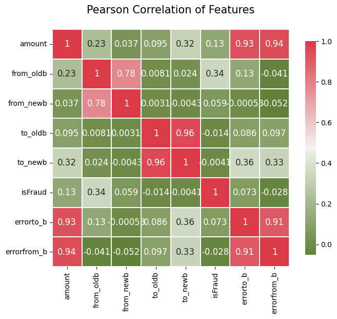
We can also use the pearson correlation to watch the relation of each two variables.

import matplotlib.pyplot as plt
import seaborn as sns
def correlation_heatmap(df):
    _ , ax = plt.subplots(figsize =(8, 6))
    colormap = sns.diverging_palette(110, 10, as_cmap = True)
    
    _ = sns.heatmap(
        df.corr(), 
        cmap = colormap,
        square=True, 
        cbar_kws={'shrink':.9 }, 
        ax=ax,
        annot=True, 
        linewidths=0.1,vmax=1.0, linecolor='white',
        annot_kws={'fontsize':12 }
    )
    
    plt.title('Pearson Correlation of Features', y=1.05, size=15)

correlation_heatmap(df)

../../_images/e4b07cecd6c04d21756b57e2b3fb86cc7320f10757550b7667abfb8f7354b9e8.png

4.model building#

X=df.drop(['isFraud'],axis=1).copy()

Y = df['isFraud']

Xgboost#

Xgboost is a machine learning tool to predict outcomes. Why I want to put it at the first place is that it can handle the missing values easily, and quicker than the random forest, and is often used in competition.

from sklearn.model_selection import train_test_split

import xgboost as xgb

For the best use of machine learning, I choose a range of learning rate to get the best prediction.

#X = pd.get_dummies(X)
X_train_xgb,X_test_xgb,y_train_xgb,y_test_xgb=train_test_split(df[['amount', 'from_oldb', 'from_newb', 'to_oldb', 'to_newb', 'errorto_b', 'errorfrom_b']],Y,test_size = 0.2,random_state=42)
answer=pd.DataFrame(columns=['i', 'train_errors', 'test_errors'])
for i in np.arange(0.05, 0.15, 0.01):
    xgbr = xgb.XGBClassifier(max_depth = 3, n_jobs = -1, random_state = 42, learning_rate = i)
    xgbr.fit(X_train_xgb, y_train_xgb)
    train_error_xgb = 1 - xgbr.score(X_train_xgb, y_train_xgb)
    test_error_xgb = 1 - xgbr.score(X_test_xgb, y_test_xgb)
    answer = answer.append({
        'i': i,
        'train_errors': train_error_xgb,
        'test_errors': test_error_xgb
    },ignore_index=True)

answer.head(5)

	i	train_errors	test_errors
0	0.05	0.000582	0.000534
1	0.06	0.000582	0.000534
2	0.07	0.000579	0.000530
3	0.08	0.000572	0.000537
4	0.09	0.000556	0.000527

answer

	i	train_errors	test_errors
0	0.05	0.000582	0.000534
1	0.06	0.000582	0.000534
2	0.07	0.000579	0.000530
3	0.08	0.000572	0.000537
4	0.09	0.000556	0.000527
5	0.10	0.000553	0.000516
6	0.11	0.000546	0.000520
7	0.12	0.000535	0.000510
8	0.13	0.000540	0.000510
9	0.14	0.000520	0.000510

import altair as alt

c1 = alt.Chart(answer).mark_line(color='black').encode(
    x='i',
    y=alt.Y('train_errors', scale=alt.Scale(domain=[0.0005, max(answer['train_errors'])]))
)


c2 = alt.Chart(answer).mark_line(color='red').encode(
    x='i',
    y=alt.Y('test_errors', scale=alt.Scale(domain=[0.0005, max(answer['test_errors'])])),
    tooltip='i'
).properties(
    title='Train Error and Test Error Depending on Learning Rate'
)


final_chart = c1 + c2
final_chart

I will use i=0.1 as the learning rate since it’s the lowest rate except the end.

xgbr = xgb.XGBClassifier(max_depth = 3, n_jobs = -1, random_state = 42, learning_rate = 0.1)
xgbr.fit(X_train_xgb, y_train_xgb)

XGBClassifier(base_score=None, booster=None, callbacks=None,
              colsample_bylevel=None, colsample_bynode=None,
              colsample_bytree=None, device=None, early_stopping_rounds=None,
              enable_categorical=False, eval_metric=None, feature_types=None,
              gamma=None, grow_policy=None, importance_type=None,
              interaction_constraints=None, learning_rate=0.1, max_bin=None,
              max_cat_threshold=None, max_cat_to_onehot=None,
              max_delta_step=None, max_depth=3, max_leaves=None,
              min_child_weight=None, missing=nan, monotone_constraints=None,
              multi_strategy=None, n_estimators=None, n_jobs=-1,
              num_parallel_tree=None, random_state=42, ...)

In a Jupyter environment, please rerun this cell to show the HTML representation or trust the notebook.
On GitHub, the HTML representation is unable to render, please try loading this page with nbviewer.org.

df_xgbr=pd.DataFrame(columns=["isFraud","pred"])
df_xgbr["isFraud"]=y_test_xgb
df_xgbr["pred"]=xgbr.predict(X_test_xgb)

df_xgbr = pd.DataFrame({
    "isFraud": df_xgbr["isFraud"],
    "pred": df_xgbr["pred"]
})
y_pred_xgbr = xgbr.predict(X_test_xgb)
y_pred_proba_xgbr = xgbr.predict_proba(X_test_xgb)[:, 1]
error_xgbr=(df_xgbr["isFraud"]==df_xgbr["pred"]).sum()/df_xgbr.shape[0]
error_xgbr

0.9994835293755494

Use confusion matrix to see the prediction failure.

import pandas as pd
import altair as alt
from sklearn.metrics import confusion_matrix


cm = confusion_matrix(y_test_xgb, y_pred_xgbr)


df_cm = pd.DataFrame(cm, index=["0", "1"], columns=["0", "1"])

df_cm_long = df_cm.reset_index().melt(id_vars='index')

chart = alt.Chart(df_cm_long).mark_text(size=20).encode(
    x='variable:N',
    y='index:N',
    color='value:Q',
    text='value:Q'
).properties(
    width=300,
    height=300,
    title='Confusion Matrix'
)

chart.display()

Logistic Regression#

from sklearn.linear_model import LogisticRegression

Logistic Regression has no need to test the parameters, just use it to classify, so it may be has the worst prediction, we can later use methods to find out.

X_train_log,X_test_log,y_train_log,y_test_log=train_test_split(df[['amount', 'from_oldb', 'from_newb', 'to_oldb', 'to_newb', 'errorto_b', 'errorfrom_b']],Y,test_size = 0.2,random_state=42)
log = LogisticRegression(random_state = 42)
log.fit(X_train_log, y_train_log)
df_log=pd.DataFrame(columns=["isFraud","pred"])
df_log["isFraud"]=y_test_log
df_log["pred"]=log.predict(X_test_log)
df_log = pd.DataFrame({
    "isFraud": df_log["isFraud"],
    "pred": df_log["pred"]
})
y_pred_log = log.predict(X_test_log)
y_pred_proba_log = log.predict_proba(X_test_log)[:, 1]
error_log=(df_log["isFraud"]==df_log["pred"]).sum()/df_log.shape[0]
error_log

0.995488577790395

import pandas as pd
import altair as alt
import seaborn as sns
from sklearn.metrics import confusion_matrix

cm = confusion_matrix(y_test_log, y_pred_log) 


df_cm = pd.DataFrame(cm, index=["0", "1"], columns=["0", "1"])

df_cm_long = df_cm.reset_index().melt(id_vars='index')

chart = alt.Chart(df_cm_long).mark_text(size=20).encode(
    x='variable:N',
    y='index:N',
    color='value:Q',
    text='value:Q'
).properties(
    width=300,
    height=300,
    title='Confusion Matrix'
)

chart.display()

random forest#

from sklearn.ensemble import RandomForestClassifier

Random forest takes much more time to estimate, we firstly set to find the best n_estimators, it may take about 5-10 min to complete.

X_train_rfc,X_test_rfc,y_train_rfc,y_test_rfc=train_test_split(df[['amount', 'from_oldb', 'from_newb', 'to_oldb', 'to_newb', 'errorto_b', 'errorfrom_b']],Y,test_size = 0.2,random_state=42)
answer_rf=pd.DataFrame(columns=['i', 'train_errors', 'test_errors'])
for i in np.arange(10, 20, 1):
    rfc = RandomForestClassifier(n_estimators = i, n_jobs = -1)
    rfc.fit(X_train_rfc, y_train_rfc)
    train_error = 1 - rfc.score(X_train_rfc, y_train_rfc)
    test_error = 1 - rfc.score(X_test_rfc, y_test_rfc)
    answer_rf = answer_rf.append({
        'i': i,
        'train_errors': train_error,
        'test_errors': test_error
    },ignore_index=True)

answer_rf.head(5)

	i	train_errors	test_errors
0	10.0	8.550853e-07	0.000010
1	11.0	0.000000e+00	0.000017
2	12.0	0.000000e+00	0.000010
3	13.0	8.550853e-07	0.000014
4	14.0	8.550853e-07	0.000014

answer_rf

	i	train_errors	test_errors
0	10.0	8.550853e-07	0.000017
1	11.0	8.550853e-07	0.000010
2	12.0	0.000000e+00	0.000010
3	13.0	0.000000e+00	0.000010
4	14.0	8.550853e-07	0.000014
5	15.0	0.000000e+00	0.000014
6	16.0	0.000000e+00	0.000014
7	17.0	8.550853e-07	0.000010
8	18.0	8.550853e-07	0.000014
9	19.0	0.000000e+00	0.000017

import altair as alt

c3 = alt.Chart(answer_rf).mark_line(color='black').encode(
    x='i',
    y='train_errors'
)


c4 = alt.Chart(answer_rf).mark_line(color='red').encode(
    x='i',
    y='test_errors',
    tooltip='i'
).properties(
    title='Train Error and Test Error Depending on n_estimators'
)


final_chart = c3 + c4
final_chart

I will choose n_estimators=15.

rfc = RandomForestClassifier(n_estimators = 15, n_jobs = -1)
rfc.fit(X_train_rfc, y_train_rfc)
df_rfc=pd.DataFrame(columns=["isFraud","pred"])
df_rfc["isFraud"]=y_test_rfc
df_rfc["pred"]=rfc.predict(X_test_rfc)
df_rfc = pd.DataFrame({
    "isFraud": df_rfc["isFraud"],
    "pred": df_rfc["pred"]
})
y_pred_rfc = rfc.predict(X_test_rfc)
y_pred_proba_rfc = rfc.predict_proba(X_test_rfc)[:, 1]
error_rfc=(df_rfc["isFraud"]==df_rfc["pred"]).sum()/df_rfc.shape[0]
error_rfc

0.9999897389942162

import pandas as pd
import altair as alt
import seaborn as sns
from sklearn.metrics import confusion_matrix

cm = confusion_matrix(y_test_rfc, y_pred_rfc)  


df_cm = pd.DataFrame(cm, index=["0", "1"], columns=["0", "1"])

df_cm_long = df_cm.reset_index().melt(id_vars='index')

chart = alt.Chart(df_cm_long).mark_text(size=20).encode(
    x='variable:N',
    y='index:N',
    color='value:Q',
    text='value:Q'
).properties(
    width=300,
    height=300,
    title='Confusion Matrix'
)

chart.display()

We can roughly compare with each other about the prediction accuracy of three models, and other stuff will be disscussed in the next part.

import altair as alt
import pandas as pd


errors = pd.DataFrame({
    'Model': ['Random Forest', 'Logistic', 'XGBoost'],
    'Error Difference': [1 - error_rfc, 1 - error_log, 1 - error_xgbr]  # Differences from 1
})

# Create a horizontal bar chart
bar_chart = alt.Chart(errors).mark_bar().encode(
    y='Model:N',
    x=alt.X('Error Difference:Q', axis=alt.Axis(format='.6f')),  
    color='Model:N'
).properties(
    title='Error Difference for Models'
)

# Create text labels for the bars
text = bar_chart.mark_text(
    align='left',
    baseline='middle',
    dx=3  
).encode(
    x=alt.X('Error Difference:Q', stack='zero'), 
    y=alt.Y('Model:N'),
    text=alt.Text('Error Difference:Q', format='.6f')  
)

chart_with_text = bar_chart + text

chart_with_text

5.model evaluation#

We will use accuracy_score, precision_score, recall_score,F1 score and AUC-ROC to decide whether it’s a good model. accuracy_score: This measures the overall correctness of the model by calculating the ratio of correctly predicted instances (both true positives and true negatives) to the total number of instances. A higher accuracy is better, but this metric can be misleading if the class distribution is imbalanced.

precision_score: Precision assesses the model’s ability to correctly identify only relevant instances. It is the ratio of true positives (correct positive predictions) to the sum of true and false positives (all positive predictions). A higher precision score is better and means fewer false positive errors.

recall_score: Recall (or sensitivity) measures the model’s ability to detect all relevant instances. It is the ratio of true positives to the sum of true positives and false negatives (all actual positive instances). A higher recall score is better, indicating fewer false negative errors.

f1_score: The F1 score is a balanced measure that combines precision and recall. It is the harmonic mean of precision and recall, providing a single metric that accounts for both false positives and false negatives. A higher F1 score is better, indicating a balanced model in terms of precision and recall.

roc_auc_score: The ROC (Receiver Operating Characteristic) AUC (Area Under the Curve) score measures a model’s ability to distinguish between the classes. It is the probability that the model ranks a randomly chosen positive instance higher than a randomly chosen negative one. A higher AUC score is better, indicating a better distinction between positive and negative instances.

from sklearn.metrics import accuracy_score, precision_score, recall_score, f1_score, roc_auc_score

XGBoost#

accuracy = accuracy_score(y_test_xgb, y_pred_xgbr)
precision = precision_score(y_test_xgb, y_pred_xgbr)
recall = recall_score(y_test_xgb, y_pred_xgbr)
f1 = f1_score(y_test_xgb, y_pred_xgbr)
auc_roc = roc_auc_score(y_test_xgb, y_pred_proba_xgbr)

print("Accuracy:", accuracy)
print("precision:", precision)
print("Recall:", recall)
print("F1 Score:", f1)
print("AUC-ROC:", auc_roc)

Accuracy: 0.9994835293755494
precision: 0.9476600985221675
Recall: 0.9588785046728971
F1 Score: 0.9532362960668938
AUC-ROC: 0.998687124019304

Logistic regression#

accuracy = accuracy_score(y_test_log, y_pred_log)
precision = precision_score(y_test_log, y_pred_log)
recall = recall_score(y_test_log, y_pred_log)
f1 = f1_score(y_test_log, y_pred_log)
auc_roc = roc_auc_score(y_test_log, y_pred_proba_log)

print("Accuracy:", accuracy)
print("precision:", precision)
print("Recall:", recall)
print("F1 Score:", f1)
print("AUC-ROC:", auc_roc)

Accuracy: 0.995488577790395
precision: 0.5688824662813102
Recall: 0.7358255451713396
F1 Score: 0.6416734582993753
AUC-ROC: 0.9495115510706759

random forest#

accuracy = accuracy_score(y_test_rfc, y_pred_rfc)
precision = precision_score(y_test_rfc, y_pred_rfc)
recall = recall_score(y_test_rfc, y_pred_rfc)
f1 = f1_score(y_test_rfc, y_pred_rfc)
auc_roc = roc_auc_score(y_test_rfc, y_pred_proba_rfc)

print("Accuracy:", accuracy)
print("precision:", precision)
print("Recall:", recall)
print("F1 Score:", f1)
print("AUC-ROC:", auc_roc)

Accuracy: 0.9999897389942162
precision: 1.0
Recall: 0.9981308411214953
F1 Score: 0.9990645463049579
AUC-ROC: 0.9990651055671961

Random forest shows the best prediction of fraud detection, and nearly all evaluation methods show the good predicition, the Xgboost is in the second place, and it shows a higher process time compared with the random forest, but presents more prediction failure, the logistic regression shows the worst result.

Summary#

Either summarize what you did, or summarize the results. Maybe 3 sentences.

In this project, we select features to predict the fraud. Firstly, we use quantitative method to get the most-related variables and feasible dataset, and then use xgboost, logistic regression and random forest to predict the fraud and their effectiveness, and shows a good result on random forest. This project can give instructions for fraud detection.

References#

Your code above should include references. Here is some additional space for references.

What is the source of your dataset(s)?

https://www.kaggle.com/datasets/ealaxi/paysim1

List any other references that you found helpful.

XGBoost: https://xgboost.readthedocs.io/en/stable/ accuracy:https://scikit-learn.org/stable/modules/model_evaluation.html#accuracy-score recall:https://scikit-learn.org/stable/modules/generated/sklearn.metrics.recall_score.html#sklearn.metrics.recall_score F1:https://scikit-learn.org/stable/modules/generated/sklearn.metrics.f1_score.html AUC-ROC:https://scikit-learn.org/stable/modules/generated/sklearn.metrics.roc_auc_score.html#sklearn.metrics.roc_auc_score confusion matrix:https://scikit-learn.org/stable/modules/model_evaluation.html#confusion-matrix

Transcation Fraud Detection

Contents

Transcation Fraud Detection#

Introduction#

1. import data#

This original dataset costs long time to process, you may switch directly to the second dataset to run the cell, it will take shorter time, this section is for simplify the dataset. You can see the instruction underneath to straightforwardly run the second csv file.#

2.EDA#

If the dataset provides too much time to process, it’s also fine to start the notebook from here.#

3.data cleaning and feature engineering#

4.model building#

Xgboost#

Logistic Regression#

random forest#

5.model evaluation#

XGBoost#

Logistic regression#

random forest#

Summary#

References#